T002 · Molecular filtering: ADME and lead-likeness criteria
Note: This talktorial is a part of TeachOpenCADD, a platform that aims to teach domain-specific skills and to provide pipeline templates as starting points for research projects.
Authors:
Michele Wichmann, CADD seminars 2017, Charité/FU Berlin
Mathias Wajnberg, CADD seminars 2018, Charité/FU Berlin
Dominique Sydow, 2018-2020, Volkamer lab, Charité
Andrea Volkamer, 2018-2020, Volkamer lab, Charité
Talktorial T002: This talktorial is part of the TeachOpenCADD pipeline described in the first TeachOpenCADD paper, comprising of talktorials T001-T010.
Aim of this talktorial
In the context of drug design, it is important to filter candidate molecules by e.g. their physicochemical properties. In this talktorial, the compounds acquired from ChEMBL (Talktorial T001) will be filtered by Lipinsik’s rule of five to keep only orally bioavailable compounds.
Contents in Theory
ADME - absorption, distribution, metabolism, and excretion
Lead-likeness and Lipinski’s rule of five (Ro5)
Radar charts in the context of lead-likeness
Contents in Practical
Define and visualize example molecules
Calculate and plot molecular properties for Ro5
Investigate compliance with Ro5
Apply Ro5 to the EGFR dataset
Visualize Ro5 properties (radar plot)
References
ADME criteria (Wikipedia and Mol Pharm. (2010), 7(5), 1388-1405)
SwissADME webserver
What are lead compounds? (Wikipedia)
What is the LogP value? (Wikipedia)
Lipinski et al. “Experimental and computational approaches to estimate solubility and permeability in drug discovery and development settings.” (Adv. Drug Deliv. Rev. (1997), 23, 3-25)
Ritchie et al. “Graphical representation of ADME-related molecule properties for medicinal chemists” (Drug. Discov. Today (2011), 16, 65-72)
[1]:
import sys

if "google.colab" in sys.modules:
    %pip install teachopencadd --no-deps -q
    !teachopencadd -d 2
    %pip uninstall teachopencadd -y -q
    %pip install -qr requirements.txt
Theory
In a virtual screening, we aim to predict whether a compound might bind to and interact with a specific target. However, if we want to identify a new drug, it is also important that this compound reaches the target and is eventually removed from the body in a favorable way. Therefore, we should also consider whether a compound is actually taken up into the body and whether it is able to cross certain barriers in order to reach its target. Is it metabolically stable and how will it be excreted once it is not acting at the target anymore? These processes are investigated in the field of pharmacokinetics. In contrast to pharmacodynamics (“What does the drug do to our body?”), pharmacokinetics deals with the question “What happens to the drug in our body?”.
ADME - absorption, distribution, metabolism, and excretion
Pharmacokinetics are mainly divided into four steps: Absorption, Distribution, Metabolism, and Excretion. These are summarized as ADME. Often, ADME also includes Toxicology and is thus referred to as ADMET or ADMETox. Below, the ADME steps are discussed in more detail (Wikipedia and Mol Pharm. (2010), 7(5), 1388-1405).
Absorption: The amount and the time of drug-uptake into the body depends on multiple factors which can vary between individuals and their conditions as well as on the properties of the substance. Factors such as (poor) compound solubility, gastric emptying time, intestinal transit time, chemical (in-)stability in the stomach, and (in-)ability to permeate the intestinal wall can all influence the extent to which a drug is absorbed after e.g. oral administration, inhalation, or contact to skin.
Distribution: The distribution of an absorbed substance, i.e. within the body, between blood and different tissues, and crossing the blood-brain barrier are affected by regional blood flow rates, molecular size and polarity of the compound, and binding to serum proteins and transporter enzymes. Critical effects in toxicology can be the accumulation of highly apolar substances in fatty tissue, or crossing of the blood-brain barrier.
Metabolism: After entering the body, the compound will be metabolized. This means that only part of this compound will actually reach its target. Mainly liver and kidney enzymes are responsible for the break-down of xenobiotics (substances that are extrinsic to the body).
Excretion: Compounds and their metabolites need to be removed from the body via excretion, usually through the kidneys (urine) or in the feces. Incomplete excretion can result in accumulation of foreign substances or adverse interference with normal metabolism.
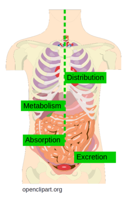
Figure 1: ADME processes in the human body (figure taken from Openclipart and adapted).
Lead-likeness and Lipinski’s rule of five (Ro5)
Lead compounds are developmental drug candidates with promising properties. They are used as starting structures and modified with the aim to develop effective drugs. Besides bioactivity (compound binds to the target of interest), also favorable ADME properties are important criteria for the design of efficient drugs.
The bioavailability of a compound is an important ADME property. Lipinski’s rule of five (Ro5, Adv. Drug Deliv. Rev. (1997), 23, 3-25) was introduced to estimate the bioavailability of a compound solely based on its chemical structure. The Ro5 states that poor absorption or permeation of a compound is more probable if the chemical structure violates more than one of the following rules:
Molecular weight (MWT) <= 500 Da
Number of hydrogen bond acceptors (HBAs) <= 10
Number of hydrogen bond donors (HBD) <= 5
Calculated LogP (octanol-water coefficient) <= 5
Note: All numbers in the Ro5 are multiples of five; this is the origin of the rule’s name.
Additional remarks:
LogP is also called partition coefficient or octanol-water coefficient. It measures the distribution of a compound, usually between a hydrophobic (e.g. 1-octanol) and a hydrophilic (e.g. water) phase.
Hydrophobic molecules might have a reduced solubility in water, while more hydrophilic molecules (e.g. high number of hydrogen bond acceptors and donors) or large molecules (high molecular weight) might have more difficulties in passing phospholipid membranes.
Radar charts in the context of lead-likeness
Molecular properties, such as the Ro5 properties, can be visualized in multiple ways (e.g. craig plots, flower plots, or golden triangle) to support the interpretation by medicinal chemists (Drug. Discov. Today (2011), 16(1-2), 65-72).
Due to their appearance, radar charts are sometimes also called “spider” or “cobweb” plots. They are arranged circularly in 360 degrees and have one axis, starting in the center, for each condition. The values for each parameter are plotted on the axis and connected with a line. A shaded area can indicate the region where the parameters meet the conditions.
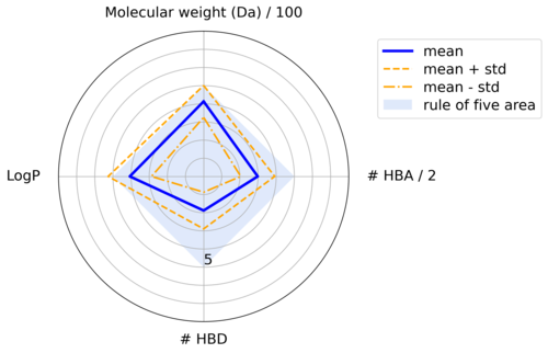
Figure 2: Radar plot displaying physico-chemical properties of a compound dataset
Practical
[2]:
from pathlib import Path
import math

import numpy as np
import pandas as pd
import matplotlib.pyplot as plt
from matplotlib.lines import Line2D
import matplotlib.patches as mpatches
from rdkit import Chem
from rdkit.Chem import Descriptors, Draw, PandasTools
[3]:
# Set path to this notebook
HERE = Path(_dh[-1])
DATA = HERE / "data"
Define and visualize example molecules
Before working with the whole dataset retrieved from ChEMBL, we pick four example compounds to investigate their chemical properties. We draw four example molecules from their SMILES.
[4]:
smiles = [
    "CCC1C(=O)N(CC(=O)N(C(C(=O)NC(C(=O)N(C(C(=O)NC(C(=O)NC(C(=O)N(C(C(=O)N(C(C(=O)N(C(C(=O)N(C(C(=O)N1)C(C(C)CC=CC)O)C)C(C)C)C)CC(C)C)C)CC(C)C)C)C)C)CC(C)C)C)C(C)C)CC(C)C)C)C",
    "CN1CCN(CC1)C2=C3C=CC=CC3=NC4=C(N2)C=C(C=C4)C",
    "CC1=C(C(CCC1)(C)C)C=CC(=CC=CC(=CC=CC=C(C)C=CC=C(C)C=CC2=C(CCCC2(C)C)C)C)C",
    "CCCCCC1=CC(=C(C(=C1)O)C2C=C(CCC2C(=C)C)C)O",
]
names = ["cyclosporine", "clozapine", "beta-carotene", "cannabidiol"]
First, we combine the names and SMILES of the molecules, together with their structure, in a DataFrame.
[5]:
molecules = pd.DataFrame({"name": names, "smiles": smiles})
PandasTools.AddMoleculeColumnToFrame(molecules, "smiles")
molecules
[5]:
| name | smiles | ROMol | |
|---|---|---|---|
| 0 | cyclosporine | CCC1C(=O)N(CC(=O)N(C(C(=O)NC(C(=O)N(C(C(=O)NC(... |  |
| 1 | clozapine | CN1CCN(CC1)C2=C3C=CC=CC3=NC4=C(N2)C=C(C=C4)C |  |
| 2 | beta-carotene | CC1=C(C(CCC1)(C)C)C=CC(=CC=CC(=CC=CC=C(C)C=CC=... |  |
| 3 | cannabidiol | CCCCCC1=CC(=C(C(=C1)O)C2C=C(CCC2C(=C)C)C)O |  |
Calculate and plot molecular properties for Ro5
Calculate molecular weight, number of hydrogen bond acceptors and donors, and logP using some of the descriptors available in
rdkit.
[6]:
molecules["molecular_weight"] = molecules["ROMol"].apply(Descriptors.ExactMolWt)
molecules["n_hba"] = molecules["ROMol"].apply(Descriptors.NumHAcceptors)
molecules["n_hbd"] = molecules["ROMol"].apply(Descriptors.NumHDonors)
molecules["logp"] = molecules["ROMol"].apply(Descriptors.MolLogP)
# Colors are used for plotting the molecules later
molecules["color"] = ["red", "green", "blue", "cyan"]
# NBVAL_CHECK_OUTPUT
molecules[["molecular_weight", "n_hba", "n_hbd", "logp"]]
[6]:
| molecular_weight | n_hba | n_hbd | logp | |
|---|---|---|---|---|
| 0 | 1201.841368 | 12 | 5 | 3.26900 |
| 1 | 306.184447 | 4 | 1 | 1.68492 |
| 2 | 536.438202 | 0 | 0 | 12.60580 |
| 3 | 314.224580 | 2 | 2 | 5.84650 |
[7]:
# Full preview
molecules
[7]:
| name | smiles | ROMol | molecular_weight | n_hba | n_hbd | logp | color | |
|---|---|---|---|---|---|---|---|---|
| 0 | cyclosporine | CCC1C(=O)N(CC(=O)N(C(C(=O)NC(C(=O)N(C(C(=O)NC(... | |
1201.841368 | 12 | 5 | 3.26900 | red |
| 1 | clozapine | CN1CCN(CC1)C2=C3C=CC=CC3=NC4=C(N2)C=C(C=C4)C | |
306.184447 | 4 | 1 | 1.68492 | green |
| 2 | beta-carotene | CC1=C(C(CCC1)(C)C)C=CC(=CC=CC(=CC=CC=C(C)C=CC=... | |
536.438202 | 0 | 0 | 12.60580 | blue |
| 3 | cannabidiol | CCCCCC1=CC(=C(C(=C1)O)C2C=C(CCC2C(=C)C)C)O | |
314.224580 | 2 | 2 | 5.84650 | cyan |
Plot the molecule properties as bar plots.
[8]:
ro5_properties = {
    "molecular_weight": (500, "molecular weight (Da)"),
    "n_hba": (10, "# HBA"),
    "n_hbd": (5, "# HBD"),
    "logp": (5, "logP"),
}
[9]:
# Start 1x4 plot frame
fig, axes = plt.subplots(figsize=(10, 2.5), nrows=1, ncols=4)
x = np.arange(1, len(molecules) + 1)
colors = ["red", "green", "blue", "cyan"]

# Create subplots
for index, (key, (threshold, title)) in enumerate(ro5_properties.items()):
    axes[index].bar([1, 2, 3, 4], molecules[key], color=colors)
    axes[index].axhline(y=threshold, color="black", linestyle="dashed")
    axes[index].set_title(title)
    axes[index].set_xticks([])

# Add legend
legend_elements = [
    mpatches.Patch(color=row["color"], label=row["name"]) for index, row in molecules.iterrows()
]
legend_elements.append(Line2D([0], [0], color="black", ls="dashed", label="Threshold"))
fig.legend(handles=legend_elements, bbox_to_anchor=(1.2, 0.8))

# Fit subplots and legend into figure
plt.tight_layout()
plt.show()
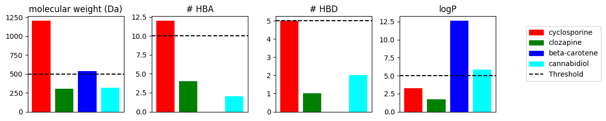
In the bar chart, we compared the Ro5 properties for four example molecules with different properties. In the next steps, we will investigate for each compound whether it violates the Ro5.
Investigate compliance with Ro5
[10]:
def calculate_ro5_properties(smiles):
    """
    Test if input molecule (SMILES) fulfills Lipinski's rule of five.

    Parameters
    ----------
    smiles : str
        SMILES for a molecule.

    Returns
    -------
    pandas.Series
        Molecular weight, number of hydrogen bond acceptors/donor and logP value
        and Lipinski's rule of five compliance for input molecule.
    """
    # RDKit molecule from SMILES
    molecule = Chem.MolFromSmiles(smiles)
    # Calculate Ro5-relevant chemical properties
    molecular_weight = Descriptors.ExactMolWt(molecule)
    n_hba = Descriptors.NumHAcceptors(molecule)
    n_hbd = Descriptors.NumHDonors(molecule)
    logp = Descriptors.MolLogP(molecule)
    # Check if Ro5 conditions fulfilled
    conditions = [molecular_weight <= 500, n_hba <= 10, n_hbd <= 5, logp <= 5]
    ro5_fulfilled = sum(conditions) >= 3
    # Return True if no more than one out of four conditions is violated
    return pd.Series(
        [molecular_weight, n_hba, n_hbd, logp, ro5_fulfilled],
        index=["molecular_weight", "n_hba", "n_hbd", "logp", "ro5_fulfilled"],
    )
[11]:
# NBVAL_CHECK_OUTPUT
for name, smiles in zip(molecules["name"], molecules["smiles"]):
    print(f"Ro5 fulfilled for {name}: {calculate_ro5_properties(smiles)['ro5_fulfilled']}")
Ro5 fulfilled for cyclosporine: False
Ro5 fulfilled for clozapine: True
Ro5 fulfilled for beta-carotene: False
Ro5 fulfilled for cannabidiol: True
According to the Ro5, cyclosporin and betacarotene are estimated to have poor bioavailability. However, since all of them are approved drugs, they are good examples of how the Ro5 can be used as an alert but should not necessarily be used as a filter.
Apply Ro5 to the EGFR dataset
The calculate_ro5_properties function can be applied to the EGFR dataset for Ro5-compliant compounds.
[12]:
molecules = pd.read_csv(DATA / "EGFR_compounds.csv", index_col=0)
print(molecules.shape)
molecules.head()
(5568, 5)
[12]:
| molecule_chembl_id | IC50 | units | smiles | pIC50 | |
|---|---|---|---|---|---|
| 0 | CHEMBL63786 | 0.003 | nM | Brc1cccc(Nc2ncnc3cc4ccccc4cc23)c1 | 11.522879 |
| 1 | CHEMBL35820 | 0.006 | nM | CCOc1cc2ncnc(Nc3cccc(Br)c3)c2cc1OCC | 11.221849 |
| 2 | CHEMBL53711 | 0.006 | nM | CN(C)c1cc2c(Nc3cccc(Br)c3)ncnc2cn1 | 11.221849 |
| 3 | CHEMBL66031 | 0.008 | nM | Brc1cccc(Nc2ncnc3cc4[nH]cnc4cc23)c1 | 11.096910 |
| 4 | CHEMBL53753 | 0.008 | nM | CNc1cc2c(Nc3cccc(Br)c3)ncnc2cn1 | 11.096910 |
Apply the Ro5 to all molecules.
[13]:
# This takes a couple of seconds
ro5_properties = molecules["smiles"].apply(calculate_ro5_properties)
ro5_properties.head()
[13]:
| molecular_weight | n_hba | n_hbd | logp | ro5_fulfilled | |
|---|---|---|---|---|---|
| 0 | 349.021459 | 3 | 1 | 5.2891 | True |
| 1 | 387.058239 | 5 | 1 | 4.9333 | True |
| 2 | 343.043258 | 5 | 1 | 3.5969 | True |
| 3 | 339.011957 | 4 | 2 | 4.0122 | True |
| 4 | 329.027607 | 5 | 2 | 3.5726 | True |
Concatenate molecules with Ro5 data.
[14]:
molecules = pd.concat([molecules, ro5_properties], axis=1)
molecules.head()
[14]:
| molecule_chembl_id | IC50 | units | smiles | pIC50 | molecular_weight | n_hba | n_hbd | logp | ro5_fulfilled | |
|---|---|---|---|---|---|---|---|---|---|---|
| 0 | CHEMBL63786 | 0.003 | nM | Brc1cccc(Nc2ncnc3cc4ccccc4cc23)c1 | 11.522879 | 349.021459 | 3 | 1 | 5.2891 | True |
| 1 | CHEMBL35820 | 0.006 | nM | CCOc1cc2ncnc(Nc3cccc(Br)c3)c2cc1OCC | 11.221849 | 387.058239 | 5 | 1 | 4.9333 | True |
| 2 | CHEMBL53711 | 0.006 | nM | CN(C)c1cc2c(Nc3cccc(Br)c3)ncnc2cn1 | 11.221849 | 343.043258 | 5 | 1 | 3.5969 | True |
| 3 | CHEMBL66031 | 0.008 | nM | Brc1cccc(Nc2ncnc3cc4[nH]cnc4cc23)c1 | 11.096910 | 339.011957 | 4 | 2 | 4.0122 | True |
| 4 | CHEMBL53753 | 0.008 | nM | CNc1cc2c(Nc3cccc(Br)c3)ncnc2cn1 | 11.096910 | 329.027607 | 5 | 2 | 3.5726 | True |
[15]:
# Note that the column "ro5_fulfilled" contains boolean values.
# Thus, we can use the column values directly to subset data.
# Note that ~ negates boolean values.
molecules_ro5_fulfilled = molecules[molecules["ro5_fulfilled"]]
molecules_ro5_violated = molecules[~molecules["ro5_fulfilled"]]

print(f"# compounds in unfiltered data set: {molecules.shape[0]}")
print(f"# compounds in filtered data set: {molecules_ro5_fulfilled.shape[0]}")
print(f"# compounds not compliant with the Ro5: {molecules_ro5_violated.shape[0]}")
# NBVAL_CHECK_OUTPUT
# compounds in unfiltered data set: 5568
# compounds in filtered data set: 4635
# compounds not compliant with the Ro5: 933
[16]:
# Save filtered data
molecules_ro5_fulfilled.to_csv(DATA / "EGFR_compounds_lipinski.csv")
molecules_ro5_fulfilled.head()
[16]:
| molecule_chembl_id | IC50 | units | smiles | pIC50 | molecular_weight | n_hba | n_hbd | logp | ro5_fulfilled | |
|---|---|---|---|---|---|---|---|---|---|---|
| 0 | CHEMBL63786 | 0.003 | nM | Brc1cccc(Nc2ncnc3cc4ccccc4cc23)c1 | 11.522879 | 349.021459 | 3 | 1 | 5.2891 | True |
| 1 | CHEMBL35820 | 0.006 | nM | CCOc1cc2ncnc(Nc3cccc(Br)c3)c2cc1OCC | 11.221849 | 387.058239 | 5 | 1 | 4.9333 | True |
| 2 | CHEMBL53711 | 0.006 | nM | CN(C)c1cc2c(Nc3cccc(Br)c3)ncnc2cn1 | 11.221849 | 343.043258 | 5 | 1 | 3.5969 | True |
| 3 | CHEMBL66031 | 0.008 | nM | Brc1cccc(Nc2ncnc3cc4[nH]cnc4cc23)c1 | 11.096910 | 339.011957 | 4 | 2 | 4.0122 | True |
| 4 | CHEMBL53753 | 0.008 | nM | CNc1cc2c(Nc3cccc(Br)c3)ncnc2cn1 | 11.096910 | 329.027607 | 5 | 2 | 3.5726 | True |
Visualize Ro5 properties (radar plot)
Calculate statistics on Ro5 properties
Define a helper function to calculate the mean and standard deviation for an input DataFrame.
[17]:
def calculate_mean_std(dataframe):
    """
    Calculate the mean and standard deviation of a dataset.

    Parameters
    ----------
    dataframe : pd.DataFrame
        Properties (columns) for a set of items (rows).

    Returns
    -------
    pd.DataFrame
        Mean and standard deviation (columns) for different properties (rows).
    """
    # Generate descriptive statistics for property columns
    stats = dataframe.describe()
    # Transpose DataFrame (statistical measures = columns)
    stats = stats.T
    # Select mean and standard deviation
    stats = stats[["mean", "std"]]
    return stats
We calculate the statistic for the dataset of compounds that are fulfilling the Ro5.
[18]:
molecules_ro5_fulfilled_stats = calculate_mean_std(
    molecules_ro5_fulfilled[["molecular_weight", "n_hba", "n_hbd", "logp"]]
)
molecules_ro5_fulfilled_stats
# NBVAL_CHECK_OUTPUT
[18]:
| mean | std | |
|---|---|---|
| molecular_weight | 414.439011 | 87.985100 |
| n_hba | 5.996548 | 1.875491 |
| n_hbd | 1.889968 | 1.008368 |
| logp | 4.070568 | 1.193034 |
We calculate the statistic for the dataset of compounds that are violating the Ro5.
[19]:
molecules_ro5_violated_stats = calculate_mean_std(
    molecules_ro5_violated[["molecular_weight", "n_hba", "n_hbd", "logp"]]
)
molecules_ro5_violated_stats
[19]:
| mean | std | |
|---|---|---|
| molecular_weight | 587.961963 | 101.999229 |
| n_hba | 7.963558 | 2.373576 |
| n_hbd | 2.301179 | 1.719732 |
| logp | 5.973461 | 1.430636 |
Define helper functions to prepare data for radar plotting
In the following, we will define a few helper functions that are only used for radar plotting.
Prepare y values: The properties used for the Ro5 criteria are of different magnitudes. The MWT has a threshold of 500, whereas the number of HBAs and HBDs and the LogP have thresholds of only 10, 5, and 5, respectively. In order to visualize these different scales most simplistically, we will scale all property values to a scaled threshold of 5:
scaled property value = property value / property threshold * scaled property threshold
scaled MWT = MWT / 500 * 5 = MWT / 100
scaled HBA = HBA / 10 * 5 = HBA / 2
scaled HBD = HBD / 5 * 5 = HBD
scaled LogP = LogP / 5 * 5 = LogP
This results in a downscaling of the MWT by 100, HBA by 2, while HBD and LogP stay unchanged.
The following helper function performs such a scaling and will be used later during radar plotting.
[20]:
def _scale_by_thresholds(stats, thresholds, scaled_threshold):
    """
    Scale values for different properties that have each an individually defined threshold.

    Parameters
    ----------
    stats : pd.DataFrame
        Dataframe with "mean" and "std" (columns) for each physicochemical property (rows).
    thresholds : dict of str: int
        Thresholds defined for each property.
    scaled_threshold : int or float
        Scaled thresholds across all properties.

    Returns
    -------
    pd.DataFrame
        DataFrame with scaled means and standard deviations for each physiochemical property.
    """
    # Raise error if scaling keys and data_stats indicies are not matching
    for property_name in stats.index:
        if property_name not in thresholds.keys():
            raise KeyError(f"Add property '{property_name}' to scaling variable.")
    # Scale property data
    stats_scaled = stats.apply(lambda x: x / thresholds[x.name] * scaled_threshold, axis=1)
    return stats_scaled
Prepare x values: The following helper function returns the angles of the physicochemical property axes for the radar chart. For example, if we want to generate a radar plot for 4 properties, we want to set the axes at 0°, 90°, 180°, and 270°. The helper function returns such angles as radians.
[21]:
def _define_radial_axes_angles(n_axes):
    """Define angles (radians) for radial (x-)axes depending on the number of axes."""
    x_angles = [i / float(n_axes) * 2 * math.pi for i in range(n_axes)]
    x_angles += x_angles[:1]
    return x_angles
Both functions will be used as helper functions in the radar plotting function, which is defined next.
Generate radar plots, finally!
Now, we define a function that visualizes the compounds’ chemical properties in the form of a radar chart. We followed these instructions on stackoverflow.
[22]:
def plot_radar(
    y,
    thresholds,
    scaled_threshold,
    properties_labels,
    y_max=None,
    output_path=None,
):
    """
    Plot a radar chart based on the mean and standard deviation of a data set's properties.

    Parameters
    ----------
    y : pd.DataFrame
        Dataframe with "mean" and "std" (columns) for each physicochemical property (rows).
    thresholds : dict of str: int
        Thresholds defined for each property.
    scaled_threshold : int or float
        Scaled thresholds across all properties.
    properties_labels : list of str
        List of property names to be used as labels in the plot.
    y_max : None or int or float
        Set maximum y value. If None, let matplotlib decide.
    output_path : None or pathlib.Path
        If not None, save plot to file.
    """

    # Define radial x-axes angles -- uses our helper function!
    x = _define_radial_axes_angles(len(y))
    # Scale y-axis values with respect to a defined threshold -- uses our helper function!
    y = _scale_by_thresholds(y, thresholds, scaled_threshold)
    # Since our chart will be circular we append the first value of each property to the end
    y = pd.concat([y, y.head(1)])

    # Set figure and subplot axis
    plt.figure(figsize=(6, 6))
    ax = plt.subplot(111, polar=True)

    # Plot data
    ax.fill(x, [scaled_threshold] * len(x), "cornflowerblue", alpha=0.2)
    ax.plot(x, y["mean"], "b", lw=3, ls="-")
    ax.plot(x, y["mean"] + y["std"], "orange", lw=2, ls="--")
    ax.plot(x, y["mean"] - y["std"], "orange", lw=2, ls="-.")

    # From here on, we only do plot cosmetics
    # Set 0° to 12 o'clock
    ax.set_theta_offset(math.pi / 2)
    # Set clockwise rotation
    ax.set_theta_direction(-1)

    # Set y-labels next to 180° radius axis
    ax.set_rlabel_position(180)
    # Set number of radial axes' ticks and remove labels
    plt.xticks(x, [])
    # Get maximal y-ticks value
    if not y_max:
        y_max = int(ax.get_yticks()[-1])
    # Set axes limits
    plt.ylim(0, y_max)
    # Set number and labels of y axis ticks
    plt.yticks(
        range(1, y_max),
        ["5" if i == scaled_threshold else "" for i in range(1, y_max)],
        fontsize=16,
    )

    # Draw ytick labels to make sure they fit properly
    # Note that we use [:1] to exclude the last element which equals the first element (not needed here)
    for i, (angle, label) in enumerate(zip(x[:-1], properties_labels)):
        if angle == 0:
            ha = "center"
        elif 0 < angle < math.pi:
            ha = "left"
        elif angle == math.pi:
            ha = "center"
        else:
            ha = "right"
        ax.text(
            x=angle,
            y=y_max + 1,
            s=label,
            size=16,
            horizontalalignment=ha,
            verticalalignment="center",
        )

    # Add legend relative to top-left plot
    labels = ("rule of five area", "mean", "mean + std", "mean - std")
    ax.legend(labels, loc=(1.1, 0.7), labelspacing=0.3, fontsize=16)

    # Save plot - use bbox_inches to include text boxes
    if output_path:
        plt.savefig(output_path, dpi=300, bbox_inches="tight", transparent=True)

    plt.show()
In the following, we want to plot the radar chart for our two datasets:
Compounds that fulfill the Ro5
Compounds that violate the Ro5
Define input parameters that should stay the same for both radar charts:
[23]:
thresholds = {"molecular_weight": 500, "n_hba": 10, "n_hbd": 5, "logp": 5}
scaled_threshold = 5
properties_labels = [
    "Molecular weight (Da) / 100",
    "# HBA / 2",
    "# HBD",
    "LogP",
]
y_max = 8
We plot the radarplot for the dataset of compounds that fulfill the Ro5.
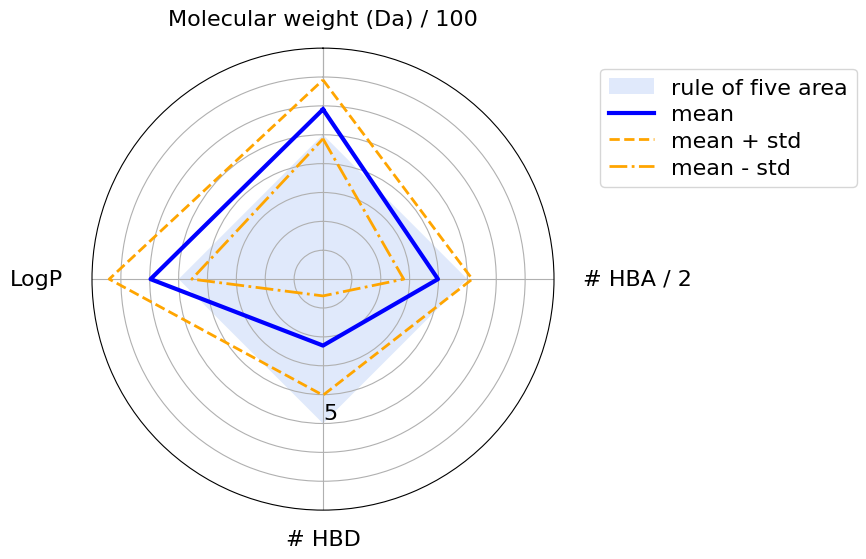
[24]:
plot_radar(
    molecules_ro5_fulfilled_stats,
    thresholds,
    scaled_threshold,
    properties_labels,
    y_max,
)
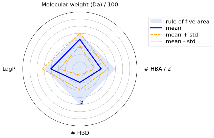
The blue square shows the area where a molecule’s physicochemical properties are compliant with the Ro5. The blue line highlights the mean values, while the orange dashed lines show the standard deviations. We can see that the mean values never violate any of Lipinski’s rules. However, according to the standard deviation, some properties have larger values then the Ro5 thresholds. This is acceptable because, according to the Ro5, one of the four rules can be violated.
We plot the radarplot for the dataset of compounds that violate the Ro5.
[25]:
plot_radar(
    molecules_ro5_violated_stats,
    thresholds,
    scaled_threshold,
    properties_labels,
    y_max,
)
We see that compounds mostly violate the Ro5 because of their logP values and their molecular weight.
Discussion
In this talktorial, we have learned about Lipinski’s Ro5 as a measure to estimate a compound’s oral bioavailability and we have applied the rule on a dataset using rdkit. Note that drugs can also be administered via alternative routes, i.e. inhalation, skin penetration and injection.
In this talktorial, we have looked at only one of many more ADME properties. Webservers such as SwissADME give a more comprehensive view on compound properties.
Quiz
In what way can the chemical properties described by the Ro5 affect ADME?
Find or design a molecule which violates three or four rules.
How can you plot information for an additional molecule in the radar charts that we have created in this talktorial?