T010 · Binding site similarity and off-target prediction
Note: This talktorial is a part of TeachOpenCADD, a platform that aims to teach domain-specific skills and to provide pipeline templates as starting points for research projects.
Authors:
Angelika Szengel, CADD seminar 2017, Charité/FU Berlin
Marvis Sydow, CADD seminar 2018, Charité/FU Berlin
Richard Gowers, RDKit UGM hackathon 2019
Jaime Rodríguez-Guerra, 2020, Volkamer lab, Charité
Dominique Sydow, 2018-2020, Volkamer lab, Charité
Mareike Leja, 2020, Volkamer lab, Charité
Talktorial T010: This talktorial is part of the TeachOpenCADD pipeline described in the first TeachOpenCADD paper, comprising of talktorials T001-T010.
Note: Please run this notebook cell by cell. Running all cells in one is possible also, however, part of the nglview 3D representations might be missing.
Aim of this talktorial
In this talktorial, we use the structural similarity of full proteins and binding sites to predict off-targets, i.e. proteins that are not intended targets of a drug. This may lead to unwanted side effects or enable desired alternate applications of a drug (drug repositioning). We discuss the main steps for binding site comparison and implement a basic method, i.e. the geometrical variation between structures (the root mean square deviation between two structures).
Contents in Theory
Off-target proteins
Computational off-target prediction: binding site comparison
Pairwise RMSD as simple measure for similarity
Imatinib, a tyrosine kinase inhibitor
Contents in Practical
Load and visualize the ligand of interest (Imatinib/STI)
Get all protein-STI complexes from the PDB
Visualize the PDB structures
Align the PDB structures (full protein)
Get pairwise RMSD (full protein)
Align the PDB structures (binding site)
Get pairwise RMSD (binding site)
Filter out outliers
References
Binding site superposition + comparison
Binding site comparison reviews:
Molecular superposition with Python:
opencaddpackage (structure.superpositionmodule) (GitHub repository)Wikipedia article on root mean square deviation (RMSD) and structural superposition
Structural superposition: Book chapter: Algorithms, Applications, and Challenges of Protein Structure Alignment in Advances in Protein Chemistry and Structural Biology (2014), 94, 121-75
Imatinib
Review on Imatinib: Nat. Rev. Clin. Oncol. (2016), 13, 431-46
Promiscuity of imatinib: J. Biol. (2009), 8, 30
Side effects of Imatinib
PDB queries
pypdbPython package Bioinformatics (2016), 1, 159-60; documentationbiotitePython package BMC Bioinformatics (2018), 19; documentationCheck out Talktorial T008 for more details on PDB queries
[1]:
import sys

if "google.colab" in sys.modules:
    %pip install teachopencadd --no-deps -q
    !teachopencadd -d 10
    %pip uninstall teachopencadd -y -q
    %pip install -qr requirements.txt
Theory
Off-target proteins
An off-target can be any protein which interacts with a drug or (one of) its metabolite(s) without being the designated target protein. The molecular reaction caused by the off-target can lead to unwanted side effects, ranging from a rather harmless to an extremely harmful impact. Off-targets mainly occur because on- and off-targets share similar structural motifs with each other in their binding site and therefore can bind similar ligands.
Computational off-target prediction: binding site comparison
Computation-aided prediction of potential off-targets is aimed at minimizing the risk of developing potentially dangerous substances for medical treatment. There are several algorithmic approaches to assess binding site similarity but they always consist of three main steps:
Binding site encoding: binding sites are encoded using different descriptor techniques and stored in a target database.
Binding site comparison: a query binding site is compared with the target database, using different similarity measures.
Target ranking: targets are ranked based on a suitable scoring approach.
For detailed information on different similarity measures and existing tools, we refer to two excellent reviews on binding site comparison (Curr. Comput. Aided Drug Des. (2008), 4, 209-20 and J. Med. Chem. (2016), 9, 4121-51).
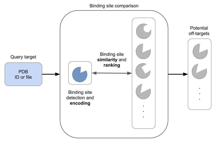
Figure 1: Main steps of binding site comparison methods (figure by Dominique Sydow).
Pairwise RMSD as simple measure for similarity
A simple and straightforward method for scoring the similarity is to use the calculated root mean square deviation (RMSD), which is the square root of the mean of the square of the distances between the atoms of two aligned structures (Wikipedia).
In order to find the respective atoms that are compared between two structures, they need to be aligned first based on sequence-based or sequence-independent alignment algorithms (Book chapter: Algorithms, Applications, and Challenges of Protein Structure Alignment in Advances in Protein Chemistry and Structural Biology (2014), 94, 121-75).
Imatinib, a tyrosine kinase inhibitor
Kinases transfer a phosphate group from ATP to proteins, and thereby regulate various cellular processes such as signal transduction, metabolism, and protein regulation. If these kinases are constitutively active (due to genomic mutations), they can distort regulation processes and cause cancer. An example for cancer treatment is Imatinib (Nat. Rev. Clin. Oncol. (2016), 13, 431-46), a small molecule tyrosine kinase inhibitor used to treat cancer, more specifically chronic myeloid leukaemia (CML) and gastrointestinal stromal tumour (GIST).
Imatinib was shown to be not entirely specific and to target tyrosine kinases other than its main target. This was used for drug repositioning, i.e. Imatinib was approved for alternate cancer types, (J. Biol. (2009), 8, 30), however can also show unwanted side effects such as signs of an allergic reaction, infection, bleeding, or headache (MedFacts Consumer Drug Information).
Practical
In the following, we will fetch and filter PDB structures that bind Imatinib. We will investigate the structure similarity of Imatinib-binding proteins (those with a solved protein structure). The similarity measure used is a pairwise RMSD calculation (as a simple similarity measure), in order to show that this simple method can be used as an initial test for potential off-targets.
[2]:
import logging
from pathlib import Path
import random
import warnings
import numpy as np
import pandas as pd
import matplotlib.pyplot as plt
import seaborn as sns
import redo
import nglview as nv
import pypdb
import biotite.database.rcsb as rcsb
from rdkit import Chem
from rdkit.Chem import Draw, AllChem
from MDAnalysis.analysis import rms
from opencadd.structure.core import Structure
from opencadd.structure.superposition.api import align, METHODS
from opencadd.structure.superposition.engines.mda import MDAnalysisAligner

SEED = 22
np.random.seed(SEED)
random.seed(SEED)
[3]:
# Ignore warnings, added because of the two following warnings
# VisibleDeprecationWarning (MDAnalysis), ClusterWarning (seaborn)
# TODO check in the future if ignoring warnings is still necessary
warnings.simplefilter("ignore")
# Also make MDAnalysis code in OpenCADD a bit less noisy
logger = logging.getLogger("opencadd")
logger.setLevel(logging.ERROR)
[4]:
# Set path to this notebook
HERE = Path(_dh[0])
DATA = HERE / "data"
[5]:
# Frozen set of PDB IDs that will be used in this notebook
# TODO check in the future if we want to update this dataset
FROZEN_PDB_IDS = ["3HEC", "2PL0", "4CSV", "4R7I", "1XBB", "3FW1", "1T46"]
Load and visualize the ligand of interest (Imatinib/STI)
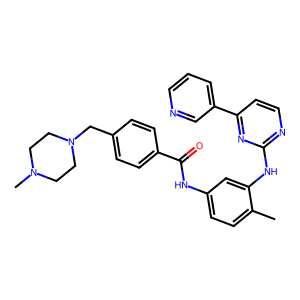
The SMILES format for Imatinib can be retrieved from e.g. the ChEMBL database by its compound ID CHEMBL941 or the PDB database by its Ligand Expo ID STI. We simply copy the string from the “Isomeric SMILES” entry of the Chemical Component Summary table, and load the ligand here by hand.
[6]:
smiles = Chem.MolFromSmiles("CN1CCN(Cc2ccc(cc2)C(=O)Nc2ccc(C)c(Nc3nccc(n3)-c3cccnc3)c2)CC1")
Draw.MolToImage(smiles)
[6]:
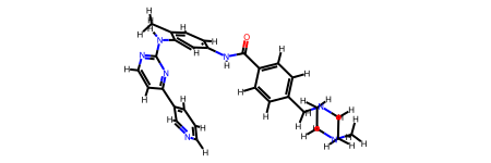
In order to inspect the 3D structure of STI, we use the open source tool nglview. Before we can view STI in nglview, we need to compute its 3D coordinates.
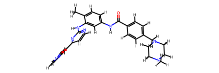
First, we add hydrogen atoms to the molecule, which are not always explicitly denoted in the SMILES format. Second, we use the distance geometry to obtain initial coordinates for the molecule and optimize the structure of the molecule using the force field UFF (Universal Force Field).
[7]:
molecule = Chem.AddHs(smiles)
molecule
[7]:
[8]:
AllChem.EmbedMolecule(molecule)
AllChem.UFFOptimizeMolecule(molecule)
molecule
[8]:
Now, we are ready to roll in nglview!
[9]:
view = nv.show_rdkit(molecule)
view
[10]:
view.render_image(trim=True, factor=2, transparent=True);
[11]:
view._display_image()
[11]:

Get protein-STI complexes from the PDB
In the following, we will search for PDB IDs describing structures in the PDB that fulfill the following criteria:
Structure is bound to Imatinib (Ligand Expo ID: STI)
Structure was experimentally resolved by X-ray crystallography
Structure has a resolution less or equal to \(3.0\)
Structure has only one chain (for simplicity)
Each structure in the PDB database is linked to many different fields to hold meta information such as our defined criteria. Check out the complete list of available fields for chemicals/structures and supported operators on the RCSB website.
The package biotite provides a very nice module databases.rcsb (see docs), which allows us to query one (FieldQuery, see docs) or more (CompositeQuery, see docs) of these
fields to retrieve a count (count) or list (search) of PDB IDs that match our criteria.
This is a table summarizing our queries:
Field |
Operator |
Value |
|---|---|---|
|
|
STI |
|
|
X-RAY DIFFRACTION |
|
|
\(3.0\) |
|
|
\(1\) |
We will first perform each of the queries alone and check the number of matches per condition. Afterwards, we will combine all queries with the and operator to match only PDB IDs that fulfill all the conditions.
Query STI-bound structures
[12]:
query_by_ligand_id = rcsb.FieldQuery(
    "rcsb_nonpolymer_entity_container_identifiers.nonpolymer_comp_id", exact_match="STI"
)
print(f"Number of matches: {rcsb.count(query_by_ligand_id)}")
Number of matches: 29
Query structures from X-ray crystallography
[13]:
query_by_experimental_method = rcsb.FieldQuery("exptl.method", exact_match="X-RAY DIFFRACTION")
print(f"Number of matches: {rcsb.count(query_by_experimental_method)}")
Number of matches: 200337
Query structures with resolution less than or equal to 3.0
[14]:
query_by_resolution = rcsb.FieldQuery("rcsb_entry_info.resolution_combined", less_or_equal=3.0)
print(f"Number of matches: {rcsb.count(query_by_resolution)}")
Number of matches: 197276
Query structures with only one chain
[15]:
query_by_polymer_count = rcsb.FieldQuery(
    "rcsb_entry_info.deposited_polymer_entity_instance_count", equals=1
)
print(f"Number of matches: {rcsb.count(query_by_polymer_count)}")
Number of matches: 85341
Query structures fulfilling all the above criteria
Use the and operator to combine the list of queries above.
[16]:
query = rcsb.CompositeQuery(
    [
        query_by_ligand_id,
        query_by_experimental_method,
        query_by_resolution,
        query_by_polymer_count,
    ],
    "and",
)
pdb_ids = rcsb.search(query)
print(f"Number of matches: {len(pdb_ids)}")
print("Selected PDB IDs:")
print(*pdb_ids)
Number of matches: 9
Selected PDB IDs:
1T46 1XBB 2PL0 3FW1 3GVU 3HEC 4CSV 4R7I 6JOL
[17]:
pdb_ids
[17]:
['1T46', '1XBB', '2PL0', '3FW1', '3GVU', '3HEC', '4CSV', '4R7I', '6JOL']
Note: The next step has technical reasons only. In order to maintain the notebooks automatically, we define here a certain set of PDB IDs to work with. Thus, even if new PDB structures matching our filtering criteria are added to the PDB, they will not be included in the downstream analysis and therefore the output will stay the same. Remote this step if you want to work with the full set of PDB structures.
[18]:
pdb_ids = FROZEN_PDB_IDS
print("Final set of PDB IDs:")
print(*pdb_ids)
Final set of PDB IDs:
3HEC 2PL0 4CSV 4R7I 1XBB 3FW1 1T46
Visualize the PDB structures
First, we load all structures in nglview for visual inspection of the 3D structure of the protein data set.
[19]:
view = nv.NGLWidget()
for pdb_id in pdb_ids:
    view.add_pdbid(pdb_id)
view
[20]:
view.render_image(trim=True, factor=2, transparent=True);
[21]:
view._display_image()
[21]:

Though this image is beautifully colorful and curly, it is not informative yet. We align the structures to each other in the next step.
[22]:
# Download PDB
structures = [Structure.from_pdbid(pdb_id) for pdb_id in pdb_ids]
# Strip solvent and other artifacts of crystallography
proteins = [Structure.from_atomgroup(s.select_atoms("protein")) for s in structures]
# Align proteins
results = align(proteins, method=METHODS["mda"])
[23]:
proteins
[23]:
[<Universe with 2684 atoms>,
 <Universe with 2182 atoms>,
 <Universe with 1968 atoms>,
 <Universe with 2269 atoms>,
 <Universe with 2124 atoms>,
 <Universe with 3648 atoms>,
 <Universe with 2381 atoms>]
Align the PDB structures (full protein)
We will use one of our opencadd packages (structure.superposition module) to guide the structural alignment of the different proteins. The approach we will use is based on superposition guided by sequence alignment provided matched residues. There are other methods in the package, but this simple one will be enough to showcase some similarities.
Note: This approach biases the analysis towards structures with similar sequences. For an automated workflow (where we do not know the sequence or structural similarity of protein pairs) a solution could be to calculate the RMSD based on all three measures and retain the best for further analysis.
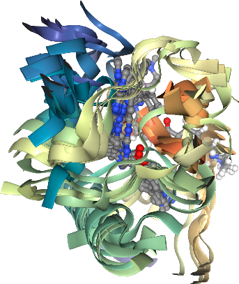
First, we show the alignment of all structures to the first structure in the our list.
[24]:
Structure.from_pdbid("4YNE")
[24]:
<Universe with 2334 atoms>
[25]:
view = nv.NGLWidget()
for protein in proteins:
    view.add_component(protein.atoms)
view
[26]:
view.render_image(trim=True, factor=2, transparent=True);
[27]:
view._display_image()
[27]:

The structural alignment for many helices is high, whereas lower or poor for other protein parts.
[28]:
def calc_rmsd(A, B):
    """
    Calculate RMSD between two structures.

    Parameters
    ----------
    A : opencadd.structure.core.Structure
        Structure A.
    B : opencadd.structure.core.Structure
        Structure B.

    Returns
    -------
    float
        RMSD value.
    """
    aligner = MDAnalysisAligner()
    selection, _ = aligner.matching_selection(A, B)
    A = A.select_atoms(selection["reference"])
    B = B.select_atoms(selection["mobile"])
    return rms.rmsd(A.positions, B.positions, superposition=False)
[29]:
def calc_rmsd_matrix(structures, names):
    """
    Calculate RMSD matrix between a list of structures.

    Parameters
    ----------
    structures : list of opencadd.structure.core.Structure
        List of structures.
    names : list of str
        List of structure names.

    Returns
    -------
    pandas.DataFrame
        RMSD matrix.
    """
    values = {name: {} for name in names}
    for i, (A, name_i) in enumerate(zip(structures, names)):
        for j, (B, name_j) in enumerate(zip(structures, names)):
            if i == j:
                values[name_i][name_j] = 0.0
                continue
            if i < j:
                rmsd = calc_rmsd(A, B)
                values[name_i][name_j] = rmsd
                values[name_j][name_i] = rmsd
                continue
    df = pd.DataFrame.from_dict(values)
    return df
Get pairwise RMSD (full protein)
[30]:
# NBVAL_CHECK_OUTPUT
rmsd_matrix = calc_rmsd_matrix(proteins, pdb_ids)
rmsd_matrix.round(1)
[30]:
| 3HEC | 2PL0 | 4CSV | 4R7I | 1XBB | 3FW1 | 1T46 | |
|---|---|---|---|---|---|---|---|
| 3HEC | 0.0 | 16.1 | 12.6 | 20.5 | 17.3 | 23.7 | 20.4 |
| 2PL0 | 16.1 | 0.0 | 3.7 | 13.5 | 7.6 | 22.8 | 16.4 |
| 4CSV | 12.6 | 3.7 | 0.0 | 14.0 | 7.8 | 22.5 | 16.7 |
| 4R7I | 20.5 | 13.5 | 14.0 | 0.0 | 11.8 | 21.9 | 8.0 |
| 1XBB | 17.3 | 7.6 | 7.8 | 11.8 | 0.0 | 22.3 | 14.3 |
| 3FW1 | 23.7 | 22.8 | 22.5 | 21.9 | 22.3 | 0.0 | 21.4 |
| 1T46 | 20.4 | 16.4 | 16.7 | 8.0 | 14.3 | 21.4 | 0.0 |
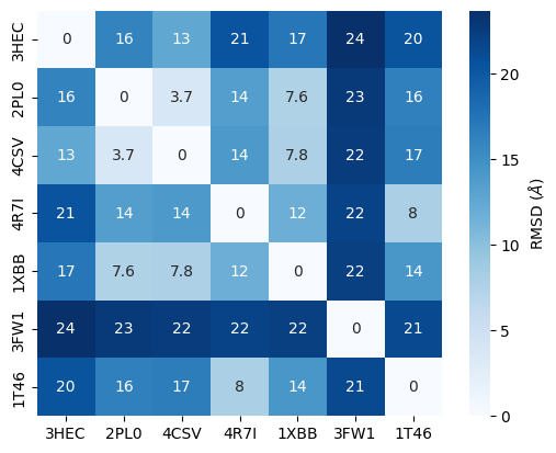
We visualize the results of this RMSD refinement as heatmap.
[31]:
# Make sure matplotlib version >= 3.1.2; otherwise you'll get Y-cropped heatmaps
sns.heatmap(
    rmsd_matrix,
    linewidths=0,
    annot=True,
    square=True,
    cbar_kws={"label": "RMSD ($\AA$)"},
    cmap="Blues",
);
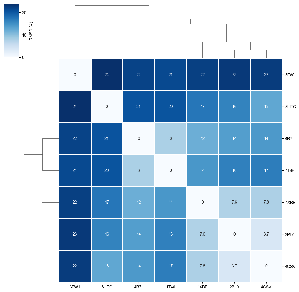
We cluster the heatmap in order to see protein similarity based on the RMSD refinement.
[32]:
def plot_clustermap(rmsd):
    """
    Plot clustered heatmap from import RMSD matrix.

    Parameters
    ----------
    rmsd : pandas.DataFrame
        RMSD matrix.
    title : str
        Plot title.

    Returns
    -------
    matplotlib.figure.Figure
        Clustered heatmap.
    """
    g = sns.clustermap(
        rmsd,
        linewidths=1,
        annot=True,
        cbar_kws={"label": "RMSD ($\AA$)"},
        cmap="Blues",
    )
    plt.setp(g.ax_heatmap.get_xticklabels(), rotation=0)
    plt.setp(g.ax_heatmap.get_yticklabels(), rotation=0)
    sns.set(font_scale=1.5)
    return plt.gcf()
[33]:
rmsd_matrix
[33]:
| 3HEC | 2PL0 | 4CSV | 4R7I | 1XBB | 3FW1 | 1T46 | |
|---|---|---|---|---|---|---|---|
| 3HEC | 0.000000 | 16.091148 | 12.589473 | 20.523115 | 17.263280 | 23.672817 | 20.421263 |
| 2PL0 | 16.091148 | 0.000000 | 3.723816 | 13.514326 | 7.557453 | 22.814496 | 16.381494 |
| 4CSV | 12.589473 | 3.723816 | 0.000000 | 14.013465 | 7.848997 | 22.471284 | 16.651349 |
| 4R7I | 20.523115 | 13.514326 | 14.013465 | 0.000000 | 11.819335 | 21.941547 | 7.951605 |
| 1XBB | 17.263280 | 7.557453 | 7.848997 | 11.819335 | 0.000000 | 22.256707 | 14.331909 |
| 3FW1 | 23.672817 | 22.814496 | 22.471284 | 21.941547 | 22.256707 | 0.000000 | 21.429275 |
| 1T46 | 20.421263 | 16.381494 | 16.651349 | 7.951605 | 14.331909 | 21.429275 | 0.000000 |
[34]:
plot_clustermap(rmsd_matrix)
[34]:

[35]:
# Check the shape of the matrix
print(f"RMSD Matrix Shape: {rmsd_matrix.shape}")

# Check for non-finite values (NaN, Inf)
print(f"Number of non-finite values: {rmsd_matrix.isna().sum().sum()}")

# Display the matrix head
print(rmsd_matrix.head())
RMSD Matrix Shape: (7, 7)
Number of non-finite values: 0
           3HEC       2PL0       4CSV       4R7I       1XBB       3FW1  \
3HEC   0.000000  16.091148  12.589473  20.523115  17.263280  23.672817
2PL0  16.091148   0.000000   3.723816  13.514326   7.557453  22.814496
4CSV  12.589473   3.723816   0.000000  14.013465   7.848997  22.471284
4R7I  20.523115  13.514326  14.013465   0.000000  11.819335  21.941547
1XBB  17.263280   7.557453   7.848997  11.819335   0.000000  22.256707

           1T46
3HEC  20.421263
2PL0  16.381494
4CSV  16.651349
4R7I   7.951605
1XBB  14.331909
The RMSD comparison shows that one protein differs most from the other proteins, i.e. 3FW1. Let’s try to understand by checking which proteins we have in our dataset.
Proteins are classified by the chemical reactions that they catalyze with EC (Enzyme Commission) numbers. We will use them here to check the enzymatic groups the proteins belong to. Let’s get the EC numbers from the PDB using the package pypdb (see more details in Talktorial T008).
[36]:
# NBVAL_CHECK_OUTPUT
# Get EC numbers for PDB IDs from PDB
pdbs_info = [pypdb.get_all_info(pdb_id) for pdb_id in pdb_ids]
# latest versions of the PDB API changed "pdbx_descriptor" to "title"
pdbx_descriptors = [pdb_info["struct"]["title"] for pdb_info in pdbs_info]
ec_numbers = pd.DataFrame(
    {
        "pdb_id": pdb_ids,
        "description": pdbx_descriptors,
    }
)
# Increase column width to fit all text
pd.set_option("max_colwidth", 100)
ec_numbers
[36]:
| pdb_id | description | |
|---|---|---|
| 0 | 3HEC | P38 in complex with Imatinib |
| 1 | 2PL0 | LCK bound to imatinib |
| 2 | 4CSV | Tyrosine kinase AS - a common ancestor of Src and Abl bound to Gleevec |
| 3 | 4R7I | Crystal structure of FMS kinase domain with a small molecular inhibitor, GLEEVEC |
| 4 | 1XBB | Crystal structure of the syk tyrosine kinase domain with Gleevec |
| 5 | 3FW1 | Quinone Reductase 2 |
| 6 | 1T46 | STRUCTURAL BASIS FOR THE AUTOINHIBITION AND STI-571 INHIBITION OF C-KIT TYROSINE KINASE |
We can see that 3FW1 is a the human quinone reductase 2 (NQO2), the only protein not belonging to class 2.7 (phosphorus transferases), which contains the tyrosine kinases (EC 2.7.10.2), the designated targets for Imatinib. 3FW1 is a reported off-target “with potential implications for drug design and treatment of chronic myelogenous leukemia in patients” (BMC Struct. Biol. (2009), 9).
Align PDB structures (binding sites)
So far, we have used the full protein structure for the alignment and RMSD refinement. However, ligands bind only at a protein’s binding site. Therefore, the similarity of binding sites is a more putative basis for off-target prediction rather than of the similarity of full protein structures.
We define a binding site of a protein by selecting all residues that are within 10 Å of any ligand atom. These binding site residues are used for alignment and only their Cɑ atoms (protein backbone) are used for the RMSD refinement. Here, we show the alignment of all structures to the first structure in our list.
Note that for the aligner to work, full residues must be selected as part of the distance search, hence the need for the same residue as (...) query.
[37]:
sel = "same residue as (resname STI or (around 10 resname STI))"
binding_sites = [Structure.from_atomgroup(s.select_atoms(sel)) for s in structures]
Let’s look at the proteins’ binding sites only.
[38]:
view = nv.NGLWidget()
for binding_site in binding_sites:
    view.add_component(binding_site.atoms)
view
[39]:
view.render_image(trim=True, factor=2, transparent=True);
[40]:
view._display_image()
[40]:
Now we align the binding sites.
[41]:
results_binding_sites = align(binding_sites, method=METHODS["mda"])
Let’s visualize our aligned binding sites.
[42]:
view = nv.NGLWidget()
for binding_site in binding_sites:
    view.add_component(binding_site.atoms)
view
[43]:
view.render_image(trim=True, factor=2, transparent=True);
[44]:
view._display_image()
[44]:

Get pairwise RMSD (binding sites)
[45]:
# NBVAL_CHECK_OUTPUT
rmsd_matrix_binding_sites = calc_rmsd_matrix(binding_sites, pdb_ids)
rmsd_matrix_binding_sites.round(1)
[45]:
| 3HEC | 2PL0 | 4CSV | 4R7I | 1XBB | 3FW1 | 1T46 | |
|---|---|---|---|---|---|---|---|
| 3HEC | 0.0 | 6.2 | 3.3 | 5.7 | 12.3 | 15.0 | 9.8 |
| 2PL0 | 6.2 | 0.0 | 4.5 | 4.0 | 11.7 | 11.3 | 4.3 |
| 4CSV | 3.3 | 4.5 | 0.0 | 5.6 | 10.7 | 14.3 | 6.3 |
| 4R7I | 5.7 | 4.0 | 5.6 | 0.0 | 10.5 | 14.5 | 2.7 |
| 1XBB | 12.3 | 11.7 | 10.7 | 10.5 | 0.0 | 13.5 | 11.1 |
| 3FW1 | 15.0 | 11.3 | 14.3 | 14.5 | 13.5 | 0.0 | 15.3 |
| 1T46 | 9.8 | 4.3 | 6.3 | 2.7 | 11.1 | 15.3 | 0.0 |
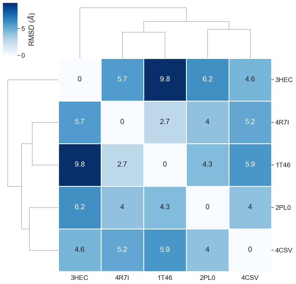
We show the clustered heatmap for the RMSD results.
[46]:
# Show the pairwise RMSD values as clustered heatmap
plot_clustermap(rmsd_matrix_binding_sites);
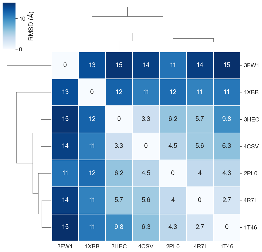
What are the key observations in this heatmap?
As observed already during the full protein comparison, also the binding site comparison reveals the highest dissimilarity for
3FW1. Since3FW1is the only structure in our dataset representing not a kinase, we are content that our similarity measure was able to spot this. As discussed before, the human quinone reductase 2 (3FW1) is a reported off-target for Imatinib.Also the kinase
1XBBshows a higher dissimilarity compared to the other kinases. This can be explained by1XBBbeing resolved in a different conformation (DFG-in) than the other kinases (DFG-out). The DFG motif is an important structural element in kinases, defining whether a kinase is active (DFG-in conformation) or inactive (DFG-out conformation). Note: DFG conformations of kinase structures can be looked up e.g. in the KLIFS database.The remaining structures are comparatively similar to each other, which we would expect since they all represent kinases in the overall same conformation.
Note that RMSD values as calculated here are dependent on the residue selection (binding site definition) and the quality of the a priori sequence alignment.
Filter out outliers
For a cleaner depiction of the most similar structures, we can filter 3FW1 and 1XBB out and re-run the binding site comparison.
[47]:
filtered_structures = []
filtered_pdb_ids = []
for name, structure in zip(pdb_ids, structures):
    if name not in ("3FW1", "1XBB"):
        filtered_structures.append(structure)
        filtered_pdb_ids.append(name)
[48]:
selection = "same residue as (resname STI or (around 10 resname STI))"
filtered_binding_sites = [
    Structure.from_atomgroup(s.select_atoms(selection)) for s in filtered_structures
]
[49]:
view = nv.NGLWidget()
for binding_site in filtered_binding_sites:
    view.add_component(binding_site.atoms)
view
[50]:
view.render_image(trim=True, factor=2, transparent=True);
[51]:
view._display_image()
[51]:
[52]:
filtered_results_binding_sites = align(filtered_binding_sites, method=METHODS["mda"])
[53]:
view = nv.NGLWidget()
for binding_site in filtered_binding_sites:
    view.add_component(binding_site.atoms)
view
[54]:
view.render_image(trim=True, factor=2, transparent=True);
[55]:
view._display_image()
[55]:

[56]:
# NBVAL_CHECK_OUTPUT
filtered_rmsd_matrix_bs = calc_rmsd_matrix(filtered_binding_sites, filtered_pdb_ids)
filtered_rmsd_matrix_bs.round(1)
[56]:
| 3HEC | 2PL0 | 4CSV | 4R7I | 1T46 | |
|---|---|---|---|---|---|
| 3HEC | 0.0 | 6.2 | 3.3 | 5.7 | 9.8 |
| 2PL0 | 6.2 | 0.0 | 4.5 | 4.0 | 4.3 |
| 4CSV | 3.3 | 4.5 | 0.0 | 5.6 | 6.3 |
| 4R7I | 5.7 | 4.0 | 5.6 | 0.0 | 2.7 |
| 1T46 | 9.8 | 4.3 | 6.3 | 2.7 | 0.0 |
[57]:
plot_clustermap(filtered_rmsd_matrix_bs);
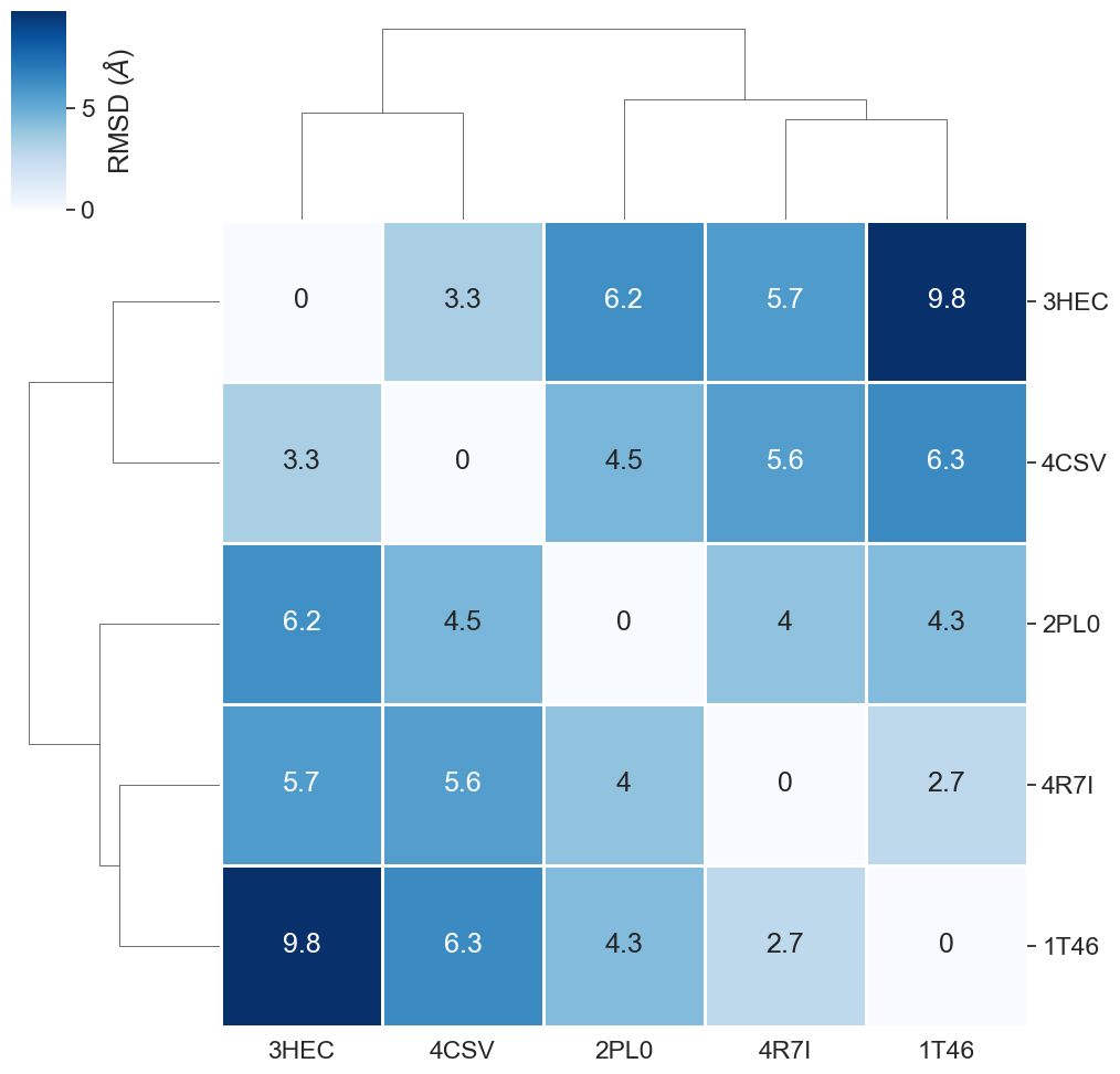
Much better!
Discussion
In this talktorial, we have used a simple comparison approach, i.e. sequence alignment and subsequent RMSD refinement of (i) full proteins and (ii) binding sites, to assess the similarity and dissimilarity of a small set of structures showing Imatinib-binding proteins. In our data set, we were able to spot an off-target for Imatinib (highest dissimilarity) and a kinase resolved in a different conformation compared to the rest of the kinases (also with a relatively high dissimilarity). Given our simple approach, we are content with these results!
In a real case scenario, off-targets for Imatinib would be predicted by comparing the binding site of an intended target of Imatinib (a tyrosine kinase) with a large database of resolved structures (PDB). Since this results in the comparison of sequences also with low similarity, more sophisticated methods should be invoked that use a sequence-independent alignment algorithm and that include the physico-chemical properties of the binding site.
Quiz
Explain the terms on- and off-targets of a drug.
Explain why binding site similarity can be used to find off-targets based on a query target.
Discuss how useful the RMSD value of (i) full proteins and (ii) protein binding sites is for off-target prediction.
Think of alternate approaches to encode binding site information.