T038 · Protein Ligand Interaction Prediction
Note: This talktorial is a part of TeachOpenCADD, a platform that aims to teach domain-specific skills and to provide pipeline templates as starting points for research projects.
Authors:
Roman Joeres, 2022, Chair for Drug Bioinformatics, UdS and HIPS, NextAID project, Saarland University
Aim of this talktorial
The goal of this talktorial is to introduce the reader to the field of protein-ligand interaction prediction using graph neural networks (GNNs). GNNs are especially useful for representing structural data such as proteins and chemical molecules (ligands) to a deep learning model. In this talktorial, we will show how to train a deep learning model to predict interactions between proteins and ligands.
Contents in Theory
Relevance of protein-ligand interaction prediction
Workflow
Biological background - proteins as graphs
Technical background
Graph Isomorphism Networks
Binary Cross Entropy Loss
Contents in Practical
Compute graph representations
Ligands to graphs
Proteins to graphs
Data Storages
Data points
Data set
Data module
Network
GNN encoder
Full model
Training routine
References
Theoretical background
Graph Neural Networks: Kipf, Welling: “Semi-Supervised Classification with Graph Convolutional Networks”, arXiv (2017) Bronstein, et al.: “Geometric deep learning: going beyond Euclidean data”, IEEE Signal Processing Magazine (2017), 4, 18-42
GNN-based Protein-Ligand Interaction Prediction: Öztürk, et al.: “DeepDTA: Deep drug-target binding affinity prediction”, Bioinformatics (2018), 34, i821-i829 Nguyen, et. al.: “GraphDTA: Predicting drug-target binding affinity with graph neural networks”, Bioinformatics (2021), 37, 1140-1147
Graph Isomorphism Network: Xu, et al.: “How powerful are graph neural networks?”, arXiv (2018)
Practical background
[1]:
import sys

if "google.colab" in sys.modules:
    %pip install teachopencadd --no-deps -q
    !teachopencadd -d 38
    %pip uninstall teachopencadd -y -q
    %pip install -qr requirements.txt
Theory
This talktorial combines several topics, you have seen in other talktorials. Here, we will describe the general idea of how to predict interactions between proteins and ligands. If some technique used in the workflow is already presented somewhere else, I’ll link to this. Otherwise, I’ll explain new things below.
Relevance of protein-ligand interaction prediction
Protein-ligand interactions are of interest in research for many reasons as can be seen in Talktorial T016. Drug discovery is one of the most important fields where interaction prediction between proteins and ligands has applications. In drug discovery, one wants to find a new drug for a given protein. Computer-aided interaction prediction helps in the process of virtual screening, where many possible ligands are tested in silico if they interact with a certain target protein. Classically, screening of potential drugs for a target protein is done in a laboratory where the candidates are manually tested and ranked by their binding affinity. The binding affinity is a measure of how strong the interaction between two molecules is. The higher the binding affinity, the stronger the interactions and the better the two molecules bind each other.
But investigating candidates manually is time-consuming and costly. Predicting binding events in a computer is way faster and cheaper. In this talktorial we will focus on predicting binding events between proteins and ligands on a qualitative level, i.e., if a protein and a ligand bind each other or not, the affinity is not interesting for now.
Model architecture
The input for our training is a dataset comprising a set of proteins and a set of ligands and a table with binding information for every pair of proteins and ligands. We will perform supervised learning (as in Talktorial T022), therefore, we split the list of interactions into a training set, a validation set, and a test set. As discussed above, we will do a binary classification of interactions, i.e., does a pair of protein and molecule interact or not?
The last component of our network architecture is a simple multilayer perceptron (MLP) as presented in Talktorial T022. The other two components are graph neural networks (GNNs) to extract features from the proteins and ligands in each pair of the dataset. As discussed in Talktorial T035 GNNs are used to compute a representation of graph-structured data that holds information about the structure. These representations are concatenated into one vector which serves as input for the final MLP.
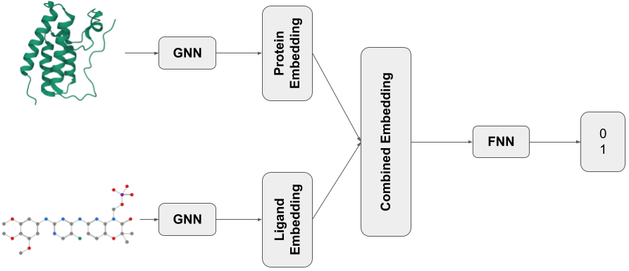
Figure 1: Visualization of the model in this notebook. The shown exemplary structures are taken from the PDB entry with ID 4O75 (see Talktorial T008 for an introduction to PDB).
Biological background - Proteins as Graphs
Here, we will focus on the conversion of proteins into graphs as the conversion of SMILES to graphs is explained in Talktorial T033.
There are usually two ways to represent proteins in science. Either by their sequence of amino acids or as a PDB structure as introduced in Talktorial T008. As amino acid sequences do not contain structural information, we use PDB files of proteins as input for our structure-based models. In the graph representation of a protein, every node of the graph represents an amino acid from the protein. Edges between nodes in the graph are drawn if the two represented amino acids are within a certain distance. This is the equivalent of an interaction between the two amino acids in the protein. To compute the distance of two amino acids, we look at the coordinates of the \(C_\alpha\) atoms of the amino acids in the PDB file. If the distance between two \(C_\alpha\) atoms is below a certain distance threshold, we consider the amino acids to interact and insert an edge in the graph representation of the protein. This can be seen in Figure 2. Atoms in amino acids are enumerated. So, \(C_\alpha\) atoms of amino acids are specific carbon atoms in each amino acid that are also present in the backbone of proteins. Examples of the \(C_\alpha\) atom in exemplary amino acids can be seen in Figures 2 and 3.
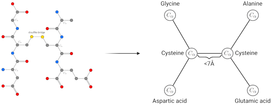
Figure 2: Visualization of the process and idea of protein structures as graphs. For this example, we consider only the \(C_\alpha\) atoms of the cysteines to be within a distance threshold of 7 Angstrom. As both cysteines are spatially close, their sulfates generate a disulfate bridge and stabilize the protein’s three-dimensions structure which is the type of interaction we want to have in the graph representations.
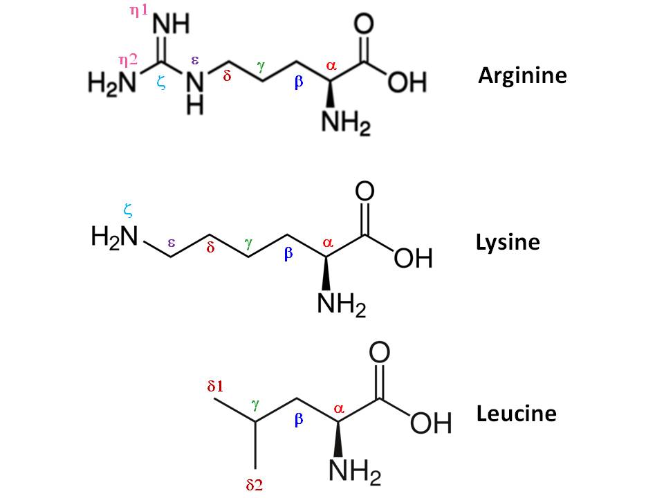
Figure 3: Visualization of carbon atoms in three exemplary amino acids. Also, other numbers for atoms in amino acids are shown, but for us, only the \(C_\alpha\) atoms are interesting (Source).
Technical background
In this section, we will focus on the computer science aspects of the proposed solution. Mainly, we will discuss the concrete GNN architecture and which node features we use. For simplicity (and because it works well), we will use the same network architecture to compute embeddings of kinases and their ligands.
Graph Isomorphism Networks
There is a whole zoo of GNN architectures proposed to solve many problems. If you want to get an overview of the most popular architectures, you can have a look at the list of convolutional layers implemented in PyTorch-Geometric. In this talktorial, we will use the GINConv layers as the backbone of out GNNs as they have been proven to be powerful in embedding molecular data yet remaining easy to understand in their functionality. The formula to compute an embedding of a node based on the neighbors is
where \(\mathcal{N}(i)\) is the set of neighbors of node \(i\), \(\epsilon\) is a constant hyperparameter, and \(h_{\mathbf{\Theta}}\) is a neural network as presented in Talktorial T022. The idea is to aggregate all neighbor embeddings together with the own current embedding and put this into a neural network to extract information on the nodes and their neighborhoods.
As can be seen, GINConv layers do not use edge information in their computation. So, the only thing we need to extract from our proteins and ligands when turning into graphs are features for the edges. In this talktorial, we will use a very simple featurization and every node just contains categorical information on the amino acid type or atom type it represents. Information on one-hot encodings of categorical data is covered in Talktorial T021.
The final element of our GNN module is the pooling function, which uses to compute the graph embedding based on the node embeddings in the final layer. For simplicity (and because it’s surprisingly powerful) we use mean pooling! That means, we just take the mean vector over all node embeddings in the final GINConv layer.
Binary Cross Entropy Loss (BCE Loss)
Talktorial T022 introduces two loss functions, namely MSE and MAE. Both are suitable to train regression models but not appropriate for classification. For classification, there is a wide range of loss functions of which we will use the Binary Cross Entropy Loss.
The formula to compute the loss is
where \(x\) is the model output for one sample and \(y\) is the label of that sample.
The idea is that exactly one term of \(y\) and \(1-y\) equals \(1\) to the formula reduces to \(\log x\) for a positive sample and \(\log (1-x)\) for a negative example. By this setting, the BCE formula ensures that you want to push the predicted values \(x\) towards 0 in negative samples (\(y=0\)) and towards \(1\) in positive cases (\(y=1\)).
For our example, positive samples (\(y=1\)) are pairs of binding kinase and ligand, then \(x\) should be close to 1. According to this, negative samples (\(y=0\)) in our example are non-binding pairs of kinase and ligand. Note the leading “-” in the formula, this flips the rest of the formula from a maximization problem to a minimization.
Practical
In this practical section, we will discuss every step in implementing the above-presented solution to protein-ligand interaction prediction. We will start with all the imports needed and some path definitions.
[2]:
import math
import random
import os
from pathlib import Path

from rdkit import Chem
import torch
import torch.nn.functional as F
from torch import nn
from torch.optim import Adam
[3]:
from torch_geometric.nn import global_mean_pool, GINConv
from torch_geometric.data import Data, InMemoryDataset
from torch_geometric.loader import DataLoader
import matplotlib.pyplot as plt

from utils import kiba_preprocessing
/home/michael/.teachopencadd_envs/teachopencadd_T038_py312/lib/python3.12/site-packages/chembl_webresource_client/__init__.py:4: UserWarning: pkg_resources is deprecated as an API. See https://setuptools.pypa.io/en/latest/pkg_resources.html. The pkg_resources package is slated for removal as early as 2025-11-30. Refrain from using this package or pin to Setuptools<81.
  __version__ = __import__('pkg_resources').get_distribution('chembl_webresource_client').version
[4]:
HERE = Path("./")
DATA = HERE / "data"
IMGS = HERE / "images"

# This method calls a data-preprocessing pipeline that is very technical and not of bigger interest for this talktorial.
# The method basically converts the KiBA dataset from an excel table to a dataset of structures in the format that we need.
kiba_preprocessing(DATA / "KIBA.csv", DATA / "resources")
KiBA originally contains 52498 ligands and 468 proteins.
KiBA after dropping sparse rows contains 79 ligands and 468 proteins.
KiBA finally contains 79 ligands and 373 proteins.
Preprocessing ligands
After ligand availability analysis KiBA contains 76 ligands and 373 proteins.
Preprocessing ligands finished
Preprocessing proteins
After protein availability analysis KiBA contains 76 ligands and 275 proteins.
Preprocessing proteins finished
Preprocessing interactions
Finally, KiBA comprises 20475 interactions.
Preprocessing interactions finished
Compute graph representations
Ligands to graphs
First, we’re going to implement the conversion of ligands into graphs. For the following explanation, the ligand has \(N\) atoms. To encode a graph, we have to compute a matrix of the node features (a \(N\times F\)-matrix where \(F\) is the number of features per node) and a matrix of the edges given by pairs of the participating node ids.
Due to some PyTorch Geometric-related implementation details, the edge matrix has to have the format \(2\times N\).
[5]:
# For every atom type we consider, map the symbol to a numerical value for one-hot encoding.
atoms_to_num = dict(
    (atom, i) for i, atom in enumerate(["C", "N", "O", "F", "P", "S", "Cl", "Br", "I"])
)


def atom_to_onehot(atom):
    """
    Return the one-hot encoding for an atom given its index in the atoms_to_num dict.

    Parameters
    ----------
    atom: str
        Atomic symbol of the atom to represent

    Returns
    -------
    torch.Tensor
        A one-hot tensor encoding the atoms features.
    """
    # initialize a 0-vector ...
    one_hot = torch.zeros(len(atoms_to_num) + 1, dtype=torch.float)
    # ... and set the according field to one, ...
    if atom in atoms_to_num:
        one_hot[atoms_to_num[atom]] = 1.0
    # ... the last field is used to represent atom types that do not have their own field in the one-hot vector
    else:
        one_hot[len(atoms_to_num)] = 1.0
    return one_hot


def smiles_to_graph(smiles):
    """
    Convert a molecule given as SDF file into a graph.

    Arguments
    ---------
    smiles: str
        Path to the file storing the structural information of the ligand

    Returns
    -------
    Tuple[torch.Tensor, torch.Tensor]
        A pair of node features and edges in the PyTorch Geometric format
    """
    # read in the molecule from an SDF file
    mol = Chem.MolFromSmiles(smiles)
    atoms, bonds = [], []
    # check if the molecule is valid
    if mol is None:
        print(smiles)
        return None, None

    # iterate over all atom, compute the feature vector and store them in a torch.Tensor object
    for atom in mol.GetAtoms():
        atoms.append(atom_to_onehot(atom.GetSymbol()))
    atoms = torch.stack(atoms)

    # iterate over all bonds in the molecule and store them in the PyTorch Geometric specific format in a torch.Tensor,
    for bond in mol.GetBonds():
        bonds.append((bond.GetBeginAtomIdx(), bond.GetEndAtomIdx()))
        bonds.append((bond.GetEndAtomIdx(), bond.GetBeginAtomIdx()))
    bonds = torch.tensor(bonds, dtype=torch.long).T

    return atoms, bonds
Proteins to graphs
Similar to how we converted ligands to graphs, we convert proteins into graphs. The output will be the same, a pair of node features and edges. To get more information on the PDB format, read this.
[6]:
# Generate a mapping from amino acids to numbers for one-hot encoding
aa_to_num = dict(
    (aa, i)
    for i, aa in enumerate(
        [
            "ALA",
            "ARG",
            "ASN",
            "ASP",
            "CYS",
            "GLU",
            "GLN",
            "GLY",
            "HIS",
            "ILE",
            "LEU",
            "LYS",
            "MET",
            "PHE",
            "PRO",
            "SER",
            "THR",
            "TRP",
            "TYR",
            "VAL",
            "UNK",
        ]
    )
)


def aa_to_onehot(aa):
    """
    Compute the one-hot vector for an amino acid representing node.

    Arguments
    ---------
    aa: str
        The three-letter code of the amino acid to be represented

    Returns
    -------
    torch.Tensor
        A one-hot tensor encoding the atoms features.
    """
    one_hot = torch.zeros(len(aa_to_num), dtype=torch.float)
    one_hot[aa_to_num[aa]] = 1.0
    return one_hot


def pdb_to_graph(pdb_file_path, max_dist=7.0):
    """
    Extract a graph representation of a protein from the PDB file.

    Arguments
    ---------
    pdb_file_path: str
        Filepath of the PDB file containing structural information on the protein
    max_dist: float
        Distance threshold to apply when computing edges between amino acids

    Returns
    -------
    Tuple[torch.Tensor, torch.Tensor]
        A pair of node features and edges in the PyTorch Geometric format
    """
    # read in the PDB file by looking for the Calpha atoms and extract their amino acid and coordinates based on the positioning in the PDB file
    residues = []
    with open(pdb_file_path, "r") as protein:
        for line in protein:
            if line.startswith("ATOM") and line[12:16].strip() == "CA":
                residues.append(
                    (
                        line[17:20].strip(),
                        float(line[30:38].strip()),
                        float(line[38:46].strip()),
                        float(line[46:54].strip()),
                    )
                )
    # Finally compute the node features based on the amino acids in the protein
    node_feat = torch.stack([aa_to_onehot(res[0]) for res in residues])

    # compute the edges of the protein by iterating over all pairs of amino acids and computing their distance
    edges = []
    for i in range(len(residues)):
        res = residues[i]
        for j in range(i + 1, len(residues)):
            tmp = residues[j]
            if math.dist(res[1:4], tmp[1:4]) <= max_dist:
                edges.append((i, j))
                edges.append((j, i))

    # store the edges in the PyTorch Geometric format
    edges = torch.tensor(edges, dtype=torch.long).T

    return node_feat, edges
Data storages
Storing and representing input data for our neural network in protein-ligand interaction prediction is a bit different from other neural networks. Therefore, we have to define our own classes to represent the data. The main difference to training an MLP as in Talktorial T008, apart from graphs being the input, is that we have two data points as input. A graph of the protein and a graph of the ligand. Therefore, we need to implement out own data infrastructure.
Data points
Usually the built-in Data class of PyTorch Geometric is used to represent only one graph, for our task, the data contains two graphs, therefore, we need to adapt the functionality to compute the number of nodes and edges for one data point.
[7]:
class DTIDataPair(Data):
    def __init__(self, **kwargs):
        super().__init__(**kwargs)

    @property
    def num_nodes(self):
        return self["lig_x"].size(0) + self["prot_x"].size(0)

    @property
    def num_edges(self):
        return self["lig_edge_index"].size(1) + self["prot_edge_index"].size(1)

    def __inc__(self, key, value, *args, **kwargs):
        """
        Method that is necessary to overwrite for successful batching of DTIDataPair object.
        In case of interest, one can look at this explanation:
        https://pytorch-geometric.readthedocs.io/en/latest/notes/batching.html

        When multiple samples are sent through a network at once, they are aggregated into batches.
        In PyTorch Geometric this is done by copying all n graphs for one batch into one graph with
        n connected components. Because of this, the node ids in the edge_index objects have to be
        changed. As they have to be increased by a fixed offset based on the number of nodes in the
        batch so far, this method computes this offset in case the edge_indices of either the
        proteins or ligands.

        Arguments
        ---------
        key: str
            String name of the field of this class to increment while batching

        Returns
        -------
        torch.Tensor
            A one-element tensor describing how to modify the values when batching.
        """
        if not key.endswith("edge_index"):
            return super().__inc__(key, value, *args, **kwargs)
        lenedg = len("edge_index")
        prefix = key[:-lenedg]
        return self[prefix + "x"].size(0)
Data set
This is where the real data magic happens. In the dataset, we read the data points and process it into the graphical representation we want to have.
[8]:
class DTIDataset(InMemoryDataset):
    def __init__(self, folder_name, file_index):
        self.folder_name = folder_name
        super().__init__(root=folder_name)
        self.data, self.slices = torch.load(self.processed_paths[file_index], weights_only=False)

    @property
    def processed_file_names(self):
        """
        Just store the names of the files where the training split, validation split, and test split are stored.

        Returns
        -------
        List[str]
            A list of filenames where the preprocessed data is stored to not recompute the preprocessing every time.
        """
        return ["train.pt", "val.pt", "test.pt"]

    def process(self):
        """
        This function is called internally in the preprocessing routine of PyTorch Geometric and defined how the dataset of PDB files, ligands, and an interaction table is converted into a dataset of graphs, ready for deep learning.
        """
        # compute all ligand graphs and store them as a dictionary with their names as key and the graphs as values
        ligand_graphs = dict()
        with open(Path(self.folder_name) / "tables" / "ligands.tsv", "r") as data:
            for line in data.readlines()[1:]:
                chembl_id, smiles = line.strip().split("\t")[:2]
                ligand_graphs[chembl_id] = smiles_to_graph(smiles)

        # compute all protein graphs and store them as a dictionary with their names as key and the graphs as values
        protein_graphs = dict(
            [
                (filename[:-4], pdb_to_graph(Path(self.folder_name) / "proteins" / filename))
                for filename in os.listdir(Path(self.folder_name) / "proteins")
            ]
        )

        with open(Path(self.folder_name) / "tables" / "inter.tsv") as inter:
            data_list = []
            for line in inter.readlines()[1:]:
                # read a line with one interaction sample. Extract ligand and protein ID and get their graphs from the dictionaries above
                protein, ligand, y = line.strip().split("\t")
                lig_node_feat, lig_edge_index = ligand_graphs[ligand]
                prot_node_feat, prot_edge_index = protein_graphs[protein]

                # if either ligand or protein are invalid graphs, skip this sample ...
                if lig_node_feat is None or prot_node_feat is None:
                    print(line.strip())
                    continue

                # ... otherwise, create a datapoint using the class from above
                data_list.append(
                    DTIDataPair(
                        lig_x=lig_node_feat,
                        lig_edge_index=lig_edge_index,
                        prot_x=prot_node_feat,
                        prot_edge_index=prot_edge_index,
                        y=torch.tensor(float(y), dtype=torch.float),
                    )
                )

            # shuffle the data, and compute how many samples go into which split
            random.shuffle(data_list)
            train_frac = int(len(data_list) * 0.7)
            test_frac = int(len(data_list) * 0.1)

            # then split the data and store them for later reuse without running the preprocessing pipeline
            train_data, train_slices = self.collate(data_list[:train_frac])
            torch.save((train_data, train_slices), self.processed_paths[0])
            val_data, val_slices = self.collate(data_list[train_frac:-test_frac])
            torch.save((val_data, val_slices), self.processed_paths[1])
            test_data, test_slices = self.collate(data_list[-test_frac:])
            torch.save((test_data, test_slices), self.processed_paths[2])
Data module
This is just a handy class holding all three splits of a dataset and providing data loaders for training, validation, and test sets.
[9]:
class DTIDataModule:
    def __init__(self, folder_name):
        self.train = DTIDataset(folder_name, 0)
        self.val = DTIDataset(folder_name, 1)
        self.test = DTIDataset(folder_name, 2)

    def train_dataloader(self):
        """
        Create and return a dataloader for the training dataset.

        Returns
        -------
        torch_geometric.loaders.DataLoader
            Dataloader on the training dataset
        """
        return DataLoader(
            self.train, batch_size=64, shuffle=True, follow_batch=["prot_x", "lig_x"]
        )

    def val_dataloader(self):
        """
        Create and return a dataloader for the validation dataset.

        Returns
        -------
        torch_geometric.loaders.DataLoader
            Dataloader on the validation dataset
        """
        return DataLoader(self.val, batch_size=64, shuffle=True, follow_batch=["prot_x", "lig_x"])

    def test_dataloader(self):
        """
        Create and return a dataloader for the test dataset.

        Returns
        -------
        torch_geometric.loaders.DataLoader
            Dataloader on the test dataset
        """
        return DataLoader(self.test, batch_size=64, shuffle=True, follow_batch=["prot_x", "lig_x"])
Network
Here, we will implement the networks as defined in the theory section.
GNN encoder
First, the GNN encoder which we will use for both, embedding proteins and embedding ligands.
[10]:
class Encoding(torch.nn.Module):
    def __init__(self, input_dim, hidden_dim=128, output_dim=64, num_layers=3):
        """
        Encoding to embed structural data using a stack of GINConv layers.

        Arguments
        ---------
        input_dim: int
            Size of the feature vector of the data
        hidden_dim: int
            Number of hidden neurons to use when computing the embeddings
        output_dim: int
            Size of the output vector of the final graph embedding after a final mean pooling
        num_layers: int
            Number of layers to use when computing embedding. This includes input and output layers, so values below 3 are meaningless.
        """
        super().__init__()
        self.layers = (
            [
                # define the input layer
                GINConv(
                    nn.Sequential(
                        nn.Linear(input_dim, hidden_dim),
                        nn.PReLU(),
                        nn.Linear(hidden_dim, hidden_dim),
                        nn.BatchNorm1d(hidden_dim),
                    )
                )
            ]
            + [
                # define a number of hidden layers
                GINConv(
                    nn.Sequential(
                        nn.Linear(hidden_dim, hidden_dim),
                        nn.PReLU(),
                        nn.Linear(hidden_dim, hidden_dim),
                        nn.BatchNorm1d(hidden_dim),
                    )
                )
                for _ in range(num_layers - 2)
            ]
            + [
                # define the output layer
                GINConv(
                    nn.Sequential(
                        nn.Linear(hidden_dim, hidden_dim),
                        nn.PReLU(),
                        nn.Linear(hidden_dim, output_dim),
                        nn.BatchNorm1d(output_dim),
                    )
                )
            ]
        )

    def forward(self, x, edge_index, batch):
        """
        Forward a batch of samples through this network to compute the forward pass.

        Arguments
        ---------
        x: torch.Tensor
            feature matrices of the graphs forwarded through the network
        edge_index: torch.Tensor
            edge indices of the graphs forwarded through the network
        batch: torch.Tensor
            Some internally used information, not relevant for the topic of this talktorial
        """
        for layer in self.layers:
            x = layer(x=x, edge_index=edge_index)
        pool = global_mean_pool(x, batch)
        return F.normalize(pool, dim=1)
Full model
Define the full model according to the workflow proposed in the theory section.
[11]:
class DTINetwork(torch.nn.Module):
    def __init__(self):
        super().__init__()

        # create encoders for both, proteins and ligands
        self.prot_encoder = Encoding(21)
        self.lig_encoder = Encoding(10)

        # define a simple FNN to compute the final prediction (to bind or not to bind)
        self.combine = torch.nn.Sequential(
            torch.nn.Linear(128, 256),
            torch.nn.ReLU(),
            torch.nn.Dropout(0.2),
            torch.nn.Linear(256, 64),
            torch.nn.ReLU(),
            torch.nn.Dropout(0.2),
            torch.nn.Linear(64, 1),
            torch.nn.Sigmoid(),
        )

    def forward(self, data):
        """
        Define the standard forward process of this network.

        Arguments
        ---------
        data: DTIDataPairBatch
            A batch of DTIDataPair samples to be predicted to train on them

        Returns
        -------
        Prediction values for all pairs in the input batch
        """
        # compute the protein embeddings using the protein embedder on the protein data of the batch
        prot_embed = self.prot_encoder(
            x=data.prot_x,
            edge_index=data.prot_edge_index,
            batch=data.prot_x_batch,
        )

        # compute the ligand embeddings using the ligand embedder on the ligand data of the batch
        lig_embed = self.lig_encoder(
            x=data.lig_x,
            edge_index=data.lig_edge_index,
            batch=data.lig_x_batch,
        )

        # concatenate both embeddings and return the output of the FNN
        combined = torch.cat((prot_embed, lig_embed), dim=1)
        return self.combine(combined)
Training routine
In the training, we will use the Adam optimizer (which is a standard choice). As described above, we use the BCE loss function to compute how far off the model’s predictions are. A special thing about the setup is that we only train for one epoch. This is because only in the first epoch the model shows improvements. After that, the model learned the dataset and does not improve much. But feel free to test more epochs. On average, one epoch takes around 10 minutes to complete.
[12]:
def train(num_epochs=1):
    """
    Implementation of the actual training routine.

    Arguments
    ---------
    num_epochs: int
        Number of epochs to train the model
    """
    # load the data, model, and define the loss function
    dataset = DTIDataModule(DATA / "resources")
    model = DTINetwork()
    loss_fn = torch.nn.BCELoss()
    optimizer = Adam(model.parameters(), lr=0.0001)
    epoch_train_acc, epoch_train_loss, epoch_val_acc, epoch_val_loss = [], [], [], []

    # train for num_epochs
    for e in range(num_epochs):
        print(f"Epoch {e + 1}/{num_epochs}")

        # perform the actual training
        train_loader = dataset.train_dataloader()
        for b, data in enumerate(train_loader):
            # compute the models predictions and the loss
            pred = model.forward(data).squeeze()
            loss = loss_fn(pred, data.y.squeeze())

            # perform one step of backpropagation
            optimizer.zero_grad()
            loss.backward()
            optimizer.step()

            # report some statistics on the training batch
            pred = pred > 0.5
            epoch_train_acc.append(sum(pred == data.y) / len(pred))
            epoch_train_loss.append(loss.item())
            print(
                f"\rTraining step {(b + 1)}/{len(train_loader)}: Loss: {epoch_train_loss[-1]:.5f}\tAcc: {epoch_train_acc[-1]:.5f}",
                end="",
            )

        torch.save(model.state_dict(), DATA / f"model_{e + 1}.pth")

        # perform validation of the last training epoch
        val_loader = dataset.val_dataloader()
        for b, data in enumerate(val_loader):
            # compute the models predictions and the loss
            pred = model.forward(data).squeeze()
            loss = loss_fn(pred, data.y.squeeze())

            # report some statistics on the validation batch
            pred = pred > 0.5
            epoch_val_acc.append(sum(pred == data.y) / len(pred))
            epoch_val_loss.append(loss.item())
            print(
                f"\rValidation step {(b + 1)}/{len(val_loader)}: Loss: {epoch_val_loss[-1]:.5f}\tAcc: {epoch_val_acc[-1]:.5f}",
                end="",
            )

    # test the final model
    print()
    test_loss, test_acc = [], []
    test_loader = dataset.test_dataloader()
    for b, data in enumerate(test_loader):
        # compute the models predictions and the loss
        pred = model.forward(data).squeeze()
        loss = loss_fn(pred, data.y.squeeze())

        # report some statistics on the validation batch
        pred = pred > 0.5
        test_acc.append(sum(pred == data.y) / len(pred))
        test_loss.append(loss.item())
        print(f"\rTesting Loss: {test_loss[-1]:.5f}\tAcc: {test_acc[-1]:.5f}", end="")
    print(
        f"\rTesting: Loss: {(sum(test_loss) / len(test_loss)):.5f}\tAcc: {(sum(test_acc) / len(test_acc)):.5f}"
    )

    fig, ax = plt.subplots(1, 2, figsize=(8, 4), sharey=True)

    ax[0].plot(epoch_train_loss, c="b", label="Train")
    ax[0].plot(
        len(epoch_train_loss) - 1, sum(epoch_val_loss) / len(epoch_val_loss), "rx", label="Val"
    )
    ax[0].set_ylim([0, 1])
    ax[0].set(xlabel="Batches")
    ax[0].set_title("Loss")

    ax[1].plot(epoch_train_acc, c="b", label="Train")
    ax[1].plot(
        len(epoch_train_loss) - 1, sum(epoch_val_loss) / len(epoch_val_loss), "rx", label="Val"
    )
    ax[1].set_ylim([0, 1])
    ax[1].set(xlabel="Batches")
    ax[1].set_title("Accuracy")

    plt.legend()
    plt.savefig(IMGS / "train_perf.png")
    plt.clf()

    return model
[13]:
!ls data/resources/processed
pre_filter.pt pre_transform.pt test.pt train.pt val.pt
/home/michael/.local/share/uv/python/cpython-3.12.8-linux-x86_64-gnu/lib/python3.12/pty.py:95: DeprecationWarning: This process (pid=33633) is multi-threaded, use of forkpty() may lead to deadlocks in the child.
  pid, fd = os.forkpty()
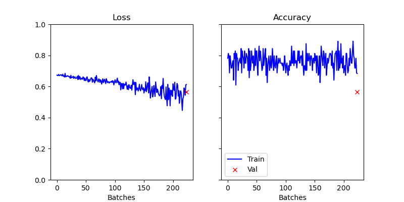
Figure 3: Visualization of the results of the first epoch of training.
Discussion
As we can see in Figure 3, the loss decreases slightly while the accuracy is stagnating. Protein-ligand interaction prediction is a highly relevant and very complex field. Due to the complexity of the binding between proteins and ligands, e.g., which atoms of the ligand bind to which site of the protein, it is difficult to train a simple model to predict these interactions. In this talktorial, we discussed a proof of concept that is further investigated in the linked literature at the beginning of this talktorial.
Quiz
With this quiz, you can test if you understand the important lessons of this talktorial.
Why do we use structural data instead of amino acid sequences and SMILES strings?
How do we convert proteins into graphs? What are the essential parts of proteins we use for that?
Difficult: Why do we need to implement our own class to represent data points?