T018 · Automated pipeline for lead optimization
Note: This talktorial is a part of TeachOpenCADD, a platform that aims to teach domain-specific skills and to provide pipeline templates as starting points for research projects.
Authors:
Armin Ariamajd, 2021, CADD seminar 2021, Charité/Freie Universität Berlin
Melanie Vogel, 2021, CADD seminar 2021, Charité/Freie Universität Berlin
Andrea Volkamer, 2021, Volkamer lab, Charité
Dominique Sydow, 2021, Volkamer lab, Charité
Corey Taylor, 2021, Volkamer lab, Charité
Aim of this talktorial
In this talktorial, we will learn how to develop an automated structure-based virtual screening pipeline. The pipeline is particularly suited for the hit expansion and lead optimization phases of a drug discovery project, where a promising ligand (i.e. an initial hit or lead compound) needs to be structurally modified in order to improve its binding affinity and selectivity for the target protein. The general architecture of the pipeline can thus be summarized as follows (Figure 1).
Input
Target protein structure and a promising ligand (e.g. lead or hit compound), plus specifications of the processes that need to be performed.
Processes
Detection of the most druggable binding site for the given protein structure.
Finding derivatives and structural analogs for the ligand, and filtering them based on drug-likeness.
Performing docking calculations on the detected protein binding site using the selected analogs.
Analyzing and vizualizing predicted protein–ligand interactions and binding modes for each analog.
Output
New ligand structure(s) optimized for affinity, selectivity and drug-likeness.
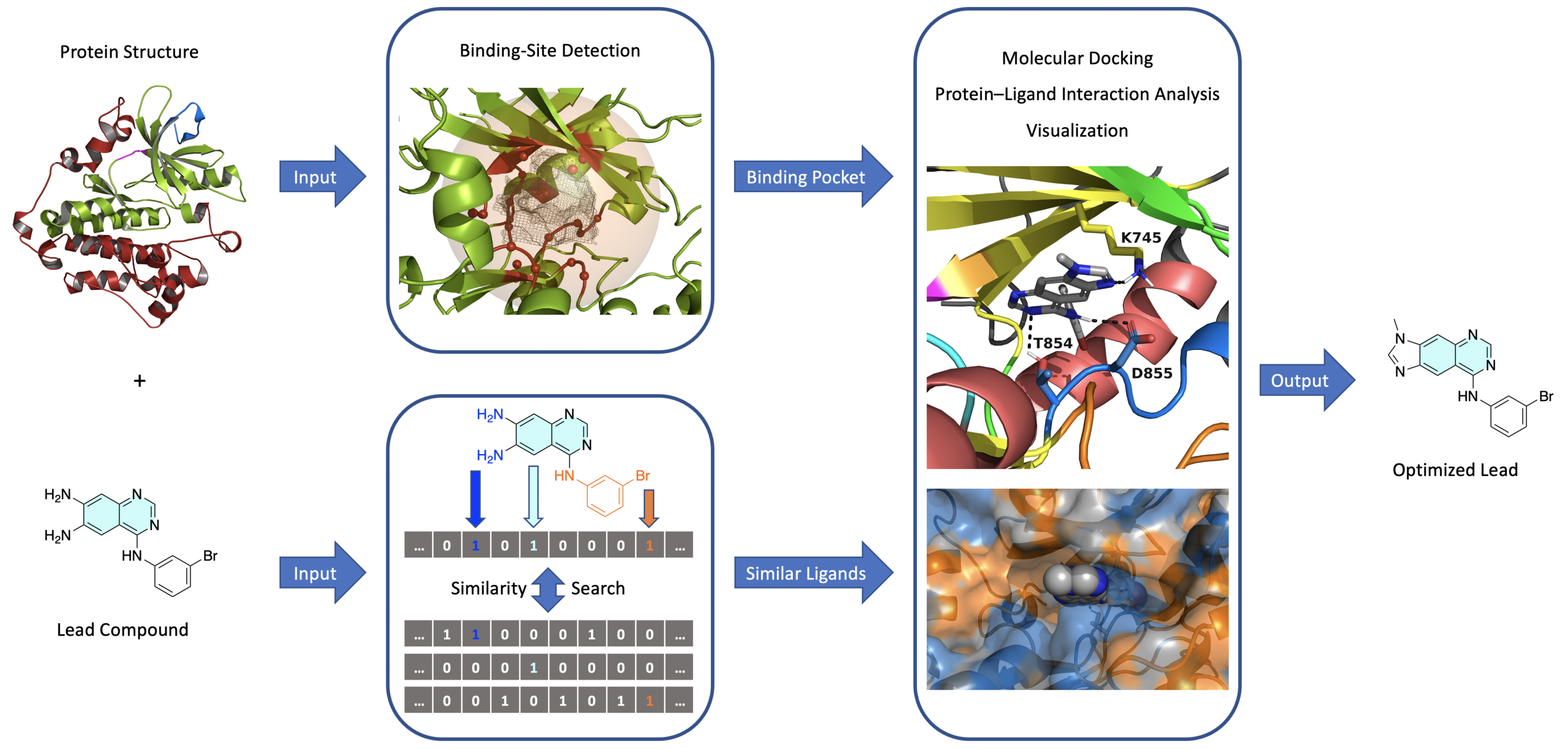
Figure 1: General architecture of the automated structure-based virtual screening pipeline.
Contents in Theory
Contents in Practical
References
Note: due to the extensive references in each category, details are hidden by default.
Click here for a complete list of references.
TeachOpenCADD teaching platform
Journal article on TeachOpenCADD teaching platform for computer-aided drug design: D. Sydow et al., J. Cheminform. 2019, 11, 29.
This talktorial is inspired by the TeachOpenCADD talktorials T013-T017
Drug design pipeline
Book on drug design: G. Klebe, Drug Design, Springer, 2013.
Review article on early stages of drug discovery: J. P. Hughes et al., Br. J. Pharmacol. 2011, 162, 1239-1249.
Review article on computational drug design: G. Sliwoski et al., Pharmacol. Rev. 2014, 66, 334-395.
Review article on computational drug discovery: S. P. Leelananda et al., Beilstein J. Org. Chem. 2016, 12, 2694-2718.
Review article on free software for building a virtual screening pipeline: E. Glaab, Brief. Bioinform. 2016, 17, 352-366.
Review article on automating drug discovery: G. Schneider, Nat. Rev. Drug Discov. 2018, 17, 97-113.
Review article on structure-based drug discovery: M. Batool et al., Int. J. Mol. Sci. 2019, 20, 2783.
Binding site detection
Book chapter on prediction and analysis of binding sites: A. Volkamer et al., Applied Chemoinformatics, Wiley, 2018, pp. 283-311.
Journal article on binding site and druggability predictions using DoGSiteScorer: A. Volkamer et al., J. Chem. Inf. Model. 2012, 52, 360-372.
Journal article describing the ProteinsPlus web-portal: R. Fahrrolfes et al., Nucleic Acids Res. 2017, 45, W337-W343.
ProteinsPlus website, and information regarding the usage of its DoGSiteScorer REST-API
TeachOpenCADD talktorial on binding site detection: Talktorial T014
TeachOpenCADD talktorial on querying online API web-services: Talktorial T011
Chemical similarity search and molecular fingerprints
Review article on molecular similarity in medicinal chemistry: G. Maggiora et al., J. Med. Chem. 2014, 57, 3186-3204.
Review article on molecular fingerprint similarity search: A. Cereto-Massague et al., Methods 2015, 71, 58-63.
Review article on molecular fingerprints in virtual screening: I. Muegge et al., *Expert Opin. Drug Discov. 2016, 11, 137-148.
Journal article on extended-connectivity fingerprints (ECFPs): D. Rogers et al., J. Chem. Inf. Model. 2010, 50, 742-754.
Journal article on Morgan algorithm: H. L. Morgan, J. Chem. Doc. 2002, 5, 107-113.
Journal article on Molecular ACCess Systems (MACCS) keys fingerprint: J. L. Durant et al., J. Chem. Inf. Comput. Sci. 2002, 42, 1273-1280.
Journal article describing the latest developments of the PubChem web-services: S. Kim et al., Nucleic Acids Res. 2019, 47, D1102-D1109.
PubChem website, and information regarding the usage of its APIs
Description of PubChem’s custom substructure fingerprint and Tanimoto similarity measure used in its similarity search engine.
TeachOpenCADD talktorial on compound similarity: Talktorial T004
TeachOpenCADD talktorial on data acquisition from PubChem: Talktorial T013
Chemical drug-likeness
Review article on drug-likeness: O. Ursu et al., Wiley Interdiscip. Rev.: Comput. Mol. Sci. 2011, 1, 760-781.
Editorial review article on drug-likeness: Nat. Rev. Drug Discov. 2007, 6, 853.
Review article on physical and chemical concepts behind drug-likeness: M. Athar et al., Phys. Sci. Rev. 2019, 4, 20180101.
Review article on available online tools for assessing drug-likeness: C. Y. Jia et al., Drug Discov. Today 2020, 25, 248-258.
Journal article on Lipinski’s rule of 5: C. A. Lipinski et al., Adv. Drug Delivery Rev. 1997, 23, 3-25.
Short review on re-assessing the rule of 5 after two decades: A. Mullard, Nat. Rev. Drug Discov. 2018, 17, 777.
Journal article on the Quantitative Estimate of Druglikeness (QED) method: G. Bickerton et al., Nat. Chem 2012, 4(2), 90-98.
RDKit documentations on calculating QED.
Molecular docking
Review article on molecular docking algorithms: X. Y. Meng et al., Curr. Comput. Aided Drug Des. 2011, 7, 146-157.
Review article on different software used for molecular docking: N. S. Pagadala et al., Biophys. Rev. 2017, 9, 91-102.
Review article on evaluation and comparison of different docking programs and scoring functions: G. L. Warren et al, J. Med. Chem. 2006, 49, 5912-5931.
Review article on evaluation of ten docking programs on a diverse set of protein-ligand complexes: Z. Wang et al., Phys. Chem. Chem. Phys. 2016, 18, 12964-12975.
Journal article describing the Smina docking program and its scoring function: D. R. Koes et al., J. Chem. Inf. Model. 2013, 53, 1893-1904.
TeachOpenCADD talktorial on protein–ligand docking: Talktorial T015
Protein-ligand interactions
Review article on protein-ligand interactions: X. Du et al., Int. J. Mol. Sci. 2016, 17, 144.
Journal article analyzing the types and frequencies of different protein-ligand interactions in available protein-ligand complex structures: R. Ferreira de Freitas et al., Med. Chem. Commun. 2017, 8, 1970-1981.
Journal article describing the PLIP algorithm: S. Salentin et al., Nucleic Acids Res. 2015, 43, W443-447.
TeachOpenCADD talktorial on protein-ligand interactions: Talktorial T016
Visual inspection of docking results
Journal article describing the NGLView program: H. Nguyen et al., Bioinformatics 2018, 34, 1241-1242.
TeachOpenCADD talktorial on advanced NGLView usage: Talktorial T017
[1]:
import sys
if "google.colab" in sys.modules:
%pip install teachopencadd --no-deps -q
!teachopencadd -d 18
%pip uninstall teachopencadd -y -q
%pip install -qr requirements.txt
%conda install openbabel plip smina -y -c conda-forge
Theory
Drug design pipeline
Modern drug discovery and development is a time and resource-intensive process comprised of several phases (Figure 2). The procedure from initial hit to the pre-clinical phase alone can take approximately two to four years and cost hundreds of millions of dollars. Causes for failure in the pre-clinical and clinical phases include compound ineffectiveness or unpredictable side-effects. Thus, computer-aided drug design pipelines can help to accelerate drug discovery projects, e.g. by prioritizing compounds.
In this talktorial, we will focus on the hit-to-lead and lead optimization phases of the pipeline: The goal is to find analogs with improved binding affinities, selectivities, physiochemical and pharmacokinetic properties.
Click here for details about the computer-aided lead optimization pipeline.
Given a target protein structure and a hit or lead compound, instead of synthesizing a variety of analogs and testing their potency in laboratory screening experiments, in a computer-aided pipeline these analogs are obtained via a similarity-search algorithm. Their physiochemical properties are then calculated to select the most drug-like analogs in order to perform docking calculations on. The result of these calculations is an estimation of the affinity of each compound for the target protein. Subsequently, analogs with the highest calculated binding affinities will be selected and their predicted binding modes are analyzed to choose those compounds that exhibit optimal protein-ligand interactions. Moreover, by filtering for specific interactions, enhanced selectivities for the target protein can be achieved as well.

Figure 2: Schematic representation of the main phases in a modern drug discovery pipeline. Figure adapted from Expert Opin. Drug. Discov. 2010, 5, 1039-1045.
Protein binding site
Binding sites, also known as binding pockets, are cavities in the 3-dimensional structure of a protein (Figure 3). These are mostly found on the surface of the protein, and are the main regions through which the protein interacts with other entities. For a favorable interaction, the two binding partners need to have complementary steric and electronic properties (cf. lock-and-key principle, induced-fit model). Therefore, attractive intermolecular interactions between the residues of the binding pocket and, for example, a small-molecule ligand is one of the key factors for molecular recognition, and thus, a ligand’s potency.
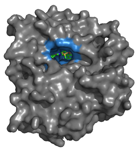
Figure 3: Crystal structure of a protein (EGFR; PDB-code: 3W32) with a co-crystallized ligand in its main (orthosteric) binding site. The protein’s surface is shown in gray. The binding site is colored blue. The ligand’s carbon atoms are colored green. Figure created using PyMol.
Binding site detection with DoGSiteScorer
For binding site detection, we will use the DoGSiteScorer functionality of the ProteinsPlus webserver. DoGSiteScorer employs a geometry- and grid-based detection algorithm where the protein is embedded into a Cartesian 3D-grid and each grid point is labeled as either free or occupied depending on whether it lies within the van-der-Waals radius of a protein atom. Subsequently, an edge-detection algorithm from image processing, called Difference of Gaussians (DoG), is used to identify protrusions on the protein surface. In doing so, cavities on the protein surface that can accommodate a spherical object are identified per grid point. Finally, cavities on neighboring grid-points are clustered together based on specific cut-off criteria, resulting in defined sub-pockets that are merged into pockets (Figure 4).
Click here for additional information on how the DoGSiteScorer algorithm works.
For each (sub-)pocket, the algorithm calculates several descriptors, e.g. volume, surface area, depth, hydrophobicity, number of hydrogen-bond donors/acceptors and amino acid count, as well as two druggability estimates (both between 0 and 1, where a higher score corresponds to a more druggable binding site):
Simple druggability score; based on a linear combination of the three descriptors for volume, hydrophobicity and enclosure.
Drug score; calculated by incorporating a subset of meaningful descriptors into a support vector machine (SVM) model, which is trained and tested on the freely available (non-redundant) druggability dataset consisting of 1069 targets.
Using these calculated descriptors and druggability estimates, we can then choose the most suitable pocket depending on the specifics of the project in hand.
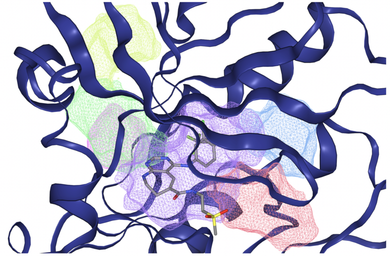
Figure 4: Visualization of some of the sub-pockets (colored meshed volumes) for the EGFR protein (PDB-code: 3W32) as detected by the DoGSiteScorer web-service. The co-crystallized ligand is mostly contained in the purple sub-pocket. Figure taken from ProteinsPlus website.
For more details see Talktorial T014 on binding site detection and the DoGSiteScorer.
Chemical similarity search
In the hit expansion and lead optimization steps of an experimental drug design pipeline, several derivatives of the initial hit/lead compound are chemically synthesized. Following the similarity hypothesis, analogues can also be computationally obtained by performing a similarity search on databases of existing chemical compounds. To do so, a numerical description of compounds is needed (Figure 5), as well as a similarity measure to compare them. One common example are molecular fingerprint descriptors together with the Tanimoto coefficient.
Click here for additional information on chemical descriptors and similarity metrics.
The simplest descriptors for a molecule are the so-called 1D-descriptors, which are scalar values corresponding to a certain property of the molecule, such as molecular weight, octanol-water partition coefficient (logP) or total polar surface area (TPSA).
However, these descriptors usually do not contain enough information to assess the structural and chemical similarity of two compounds. For this purpose, 2D-descriptors, also known as molecular fingerprints, are usually used. These descriptors are vectors that can represent a specific molecular structure in much more detail using a set of scalars.
A variety of algorithms are available for generation of 2D-descriptors from chemical structures, e.g. Molecular ACCess System (MACCS) structural keys (also known as MDL keys), and circular fingerprints, such as Extended-Connectivity FingerPrints (ECFP)/Morgan fingerprints. Generally, these algorithms work by extracting a set of specific features from the structure (Figure 5), generating a numerical representation for each feature, and using these representations to produce either a bit-vector, where each component is a bit defining the presence/absence of a particular feature (e.g. Morgan fingerprints), or a count-vector where each value corresponds to the number of times a specific feature is present in the structure (e.g. MACCS keys).
Moreover, several scoring functions are available to calculate the similarity between two molecules based on their 2D-descriptors. These include Euclidean distance and Manhattan distance, where both presence and absence of attributes are considered, or Tanimoto and Dice coefficients, which only consider the presence of attributes. It should be noted that there is no single correct approach to calculate molecular similarity, and depending on the purpose of the project different descriptors and metrics may be used, which can generally result in vastly different similarity scores.
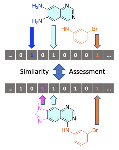
Figure 5: A simplified depiction of the process of calculating the similarity between two compounds. First, the structure of each compound is encoded into a molecular fingerprint bit-vector, where each bit corresponds to the presence or absence of a particular fragment in the structure, for example. These fingerprints can then be compared using different similarity metrics in order to calculate a similarity score.
See Talktorial T004 to become more familiar with encoding and comparison of molecular similarity measures.
PubChem database
In this talktorial, we will use the PubChem web-services for performing the similarity search on the input ligand. PubChem, which is maintained by the U.S. National Center for Biotechnology Information (NCBI) contains an open database with 110 million chemical compounds and their properties (e.g. identifiers, physiochemical properties, biological activities etc.), which can be accessed through both a web-based interface, and several different web-service Application Programming Interfaces (APIs).
Here, we will use their PUG-REST API, which allows for directly performing similarity searches on the database, using a custom substructure fingerprint as the 2D-descriptor, and the Tanimoto similarity measure as the metric. Therefore, by submitting a compound’s identifier (e.g. SMILES, CID, InChI etc.) to the PubChem’s API and providing a similarity threshold and the desired number of maximum results, a certain number of compounds within the given similarity threshold can be obtained.
For more details on data acquisition from PubChem, see Talktorial T013.
Molecular docking
After defining an appropriate binding site in the target protein and obtaining a set of analogs for the ligand of interest, the next step is to assess the suitability of each analog in terms of its position in the binding site, otherwise known as the binding mode, and its estimated fit or binding affinity. This can be done using a molecular docking algorithm.
The process works by sampling the ligand’s conformational space in the protein’s binding site and evaluating the energetics of protein-ligand interactions for each generated conformation using a scoring function. Doing so, the binding affinity of each docking pose is estimated to determine the energetically most-favorable binding modes. Examples for calculated docking poses are shown in Figure 6.
Click here for additional information on the docking process.
Most docking programs require some preparation of the protein and ligand structures. For example:
Hydrogen atoms that are usually absent in crystal structures should be added to the protein.
The correct protonation state of each atom should be calculated based on a given pH value, usually physiological pH (7.4).
Partial charges should be assigned to all atoms.
For ligands, which are usually inputted via text-based representation (e.g. SMILES), a low-energy conformer should also be generated, as the starting point in the conformational sampling process.
However, most of these calculations have some limitations; for example, they can be computationally expensive, e.g. in the case of calculating the ligand’s lowest-energy conformer, or require information that is ambiguous or not available beforehand, such as protonation states of the protein and ligand after docking. These limitations, along with others inherent in all force-field based methods, do affect the accuracy of the estimates from docking results. For example, in many cases the docking pose with the highest estimated binding affinity does not correspond to the experimentally determined binding mode of the ligand (Figure 6).
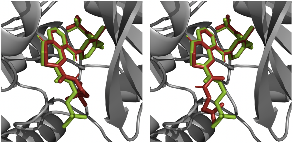
Figure 6: An example of two generated docking poses (red) in a re-docking experiment performed using the Smina program, superimposed over the corresponding protein structure (EGFR; PDB-code: 3W32) and the co-crystallized ligand in its native binding mode (green). While the generated docking pose shown on the left is calculated to have a higher binding affinity, it also displays a higher distance-RMSD to the native docking pose. Figure created using PyMol.
In this talktorial, we will use the Smina docking program, which is an open-source fork of the docking program Autodock Vina, with a focus on improved scoring functions and energy minimization. It uses a custom empirical scoring function as default but also supports user-parameterized scoring functions.
Furthermore, in order to prepare the protein and ligand structures for the docking experiment (as described above), we will also use the Pybel module of the OpenBabel package - a Python package for the Open Babel program.
For more details on protein–ligand docking, see Talktorial T015.
Protein—ligand interactions
The number and type of non-covalent intermolecular interactions between the protein and the ligand (known as protein—ligand interactions) are determining factors of the ligand’s potency. The overall affinity of a ligand is an intricate balance of several types of interactions which are mostly governed by steric and electronic properties of the interacting partners.
While the most common of these interactions are estimated by the scoring function of the docking algorithm, it is useful to explicitly analyze them in the binding modes generated by the docking calculation. This information can be used to validate the calculated binding poses, or to narrow the choice of an optimal lead compound in terms of selectivity, e.g. by choosing those derivatives that exhibit interactions with specific mutated or non-conserved residues in the protein.
In this talktorial, we will use the PLIP package - a Python package for the Protein—Ligand Interaction Profiler (PLIP), an open-source program with an available webserver. PLIP can analyze protein-ligand interactions in any given protein-ligand complex structure, by selecting pairs of atoms - one from the protein and one from the ligand - that lie within a pre-defined distance cut-off value. It then identifies the potential interactions between selected pairs based on electronic and geometric considerations.
Thus, a set of information is outputted for each detected interaction, including the interaction type, the involved atoms in both ligand and protein, along with other properties specific to each interaction type. The results can then be used to visualize the protein-ligand interactions (Figure 7) or to analyze them algorithmically.
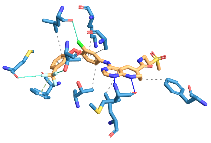
Figure 7: Visualization of the protein-ligand interactions in a protein-ligand complex structure (EGFR; PDB-code: 3W32) detected by the PLIP web-service. From the protein, only the interacting residues are shown. The protein and ligand carbon atoms are colored blue and brown, respectively. Hydrophobic interactions are shown as gray dashed lines. Hydrogen bonds are depicted as blue lines. \(\pi\)-stacking interactions are shown as green dashed lines. Halogen bonds are displayed using cyan lines. Figure taken from PLIP website.
For more details on protein-ligand interactions, see Talktorial T016.
Visual inspection of docking results
Visual inspection of the calculated docking poses and their corresponding protein—ligand interactions is inevitable. However, since manual inspection is a time-consuming process, it can only be performed on a small subset of calculated docking poses. These are usually the poses with the highest calculated binding affinities.
Some of the most common considerations when selecting a binding mode are:
Similarity to experimentally observed binding modes in available crystal structures of the target protein
Steric and electronic complementarity
Non-solvent-exposed polar functional groups in the ligand should have an interaction partner in the protein
Absence of solvent-exposed hydrophobic moieties in the ligand
Assessment of the displacement of - or interactions with - water molecules in the pocket
Steric strain induced by the ligand binding
To visualize the results, we use NGLview, a Jupyter widget using a Python wrapper for the Javascript-based NGL library. This allows for visualization of structures within a Jupyter notebook in an interactive 3D view.
For more details on advanced NGLview usage, see Talktorial T017.
Practical
In this section, we will implement and demonstrate the automated lead optimization pipeline step by step.
Technical note: The presented pipeline returns stable results for Ubuntu, MacOS, and Windows individually, however, slightly different results when comparing across different OS (for details see GH issue 191).
First, the absolute path for loading and saving the data is set.
[3]:
%load_ext autoreload
%autoreload 2
[4]:
from pathlib import Path
HERE = Path(_dh[-1])
DATA = HERE / "data"
Due to maintenance reasons, we are using frozen datasets at two steps of the pipeline that would otherwise return slightly different results each time this notebook is executed:
PubChem similarity search: Since the PubChem database is constantly updated, the similarity search results may vary . We thus use a frozen set of analogs to ensure stable results in this notebook.
Docking initial structures: Generation of PDBQT files using the
Pybelmodule (to use as starting point for the docking experiments) will unavoidably result in different atomic coordinates each time (see this discussion). By employing a set of pre-generated PDBQT files we thus ensure stable docking results.
If you wish to run this notebook without frozen data, please set USE_FROZEN_DATASETS to False in the cell below.
[5]:
# If you want to unfreeze the datasets, please set `USE_FROZEN_DATASETS` to False
USE_FROZEN_DATASETS = True
[6]:
from utils import FrozenData
frozen_data_project1 = FrozenData("Project1", USE_FROZEN_DATASETS)
frozen_data_project2 = FrozenData("Project2", USE_FROZEN_DATASETS)
Outline of the virtual screening pipeline
As this is a relatively large project with several different functionalities, it is a good practice to use classes. We are going to organize these classes into a processing sequence analogous to a pipeline, which is very useful for organizing the program by form and function. In doing so, the code will be well-structured and easier to follow, maintain, reuse, and expand upon.
Click here for additional information on the use of classes, methods, attributes and objects in Object-Oriented Programming.
A class is a code template usually consisting of a number of functions (called methods) and variables (called attributes), or even other classes (called sub-classes). This template is used to create dynamic pieces of program, called objects, with certain behaviors and properties, which are implemented by the methods and attributes defined in the class, respectively.
At any given point in the program’s runtime, an object is in a specific state, determined by the values of the object’s attributes. The methods available to the object can then be used to change the state of the object, either by changing the value of its existing attributes, or by creating new ones.
A class can be used to create any number of objects in a process called instantiation. Each object is thus an instance of the class that was used to create it. Instantiation is usually performed by providing a set of specific values for the initial state of the object. Thus all objects created from the same class will have the same types of behavior and properties, but they can be in different states.
A typical example would be a class called Car, which can be used to create car objects. The Car class may have attributes such as manufacturer, model, zero_to_hundred and current_speed, and methods like accelerate and break. By providing these attributes we can instantiate the Car class, for example to create two car objects: a Lamborghini Veneno with a zero-to-hundred of 3 seconds, and a Ford Mustang with a zero-to-hundred of 5 seconds. Let’s say we
set the current speed of both cars to 0 kmph. Now by calling the accelerate method of each car, we can change that car object’s state, i.e. its current_speed attribute. Moreover, the value of current_speed after a given amount of time would depend on the value of the car object’s zero_to_hundred attribute. For example, in the case of the Lamborghini Veneno it will become 100 kmph after 3 seconds, whereas for the Ford Mustang it will reach the same value after 5
seconds.
Another more relevant example that is also used in this pipeline is a Ligand class, which can be used to create different ligand objects. We can instantiate the class by providing a ligand’s identifier, such as SMILES. The created object will thus have a smiles attribute. Methods of the Ligand class can then be used, for example to create other attributes for the ligand, e.g. its IUPAC name, molecular weight, or a drug-likeness score. We
can also implement methods, e.g. to visualize the structure of the ligand, prepare the ligand for docking by adding hydrogen atoms and creating a 3D conformation, and to save it to a file.
As you can see, an object is a versatile representation; it can be passed between points in the program for further use or processing, depending on what type of object it is or which class created it. Classes and objects are the essence of all Object-Oriented Programming (OOP) languages, such as Python.
As a first step, we will define a class LeadOptimizationPipeline as a container for our project, and instantiate it with only a single attribute called name. For the rest of the talktorial, we will use the eight main classes of the pipeline shown below (Figure 8), instantiate them with the necessary input data, and assign those instances to our created project, so that we will have all the generated data for our project inside a single object.
While it is not necessary that the main classes are defined in a specific order, you will see as we go that we can often reuse the functionality from one created object in another. Thus, a natural order forms (Specs followed by Protein followed by Ligand etc.).
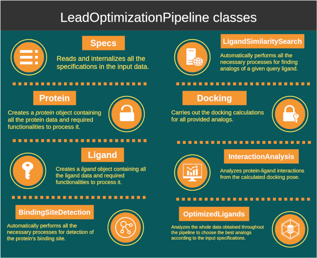
Figure 8: Main classes used in the pipeline of this talktorial.
As the code behind each class contains dozens of lines, we will not present all of it in this notebook directly. These classes are stored in a separate folder (utils) and will be imported and used as necessary. Feel free to peruse those files if you would like to know more about the exact operations that are being done when the code is executed. It bears pointing out that one is not limited to the methods implemented for this talktorial; one of the key advantages of writing a pipeline in
this manner is that you can easily add more functionality yourself.
Furthermore, most of the above classes rely on several helper modules (e.g. io, pdb, pubchem), which contain functionalities to assist in the operations of the main classes, such as retrieving data or implementing the software needed to perform a task. These helper modules are stored in a separate folder as well (utils/helpers), and can be easily adopted for reuse in other related programs.
Click here for additional information on helper modules that are implemented in this talktorial.
The ``Consts`` class
To allow for a more robust pipeline, we define a data class called Consts, which contains all the possible keywords in the input dataframe, such as the column names, index names, subject names, properties, etc. These keywords are all stored in their respective sub-classes as enumerations, so that the rest of the code needs only to refer to the enumeration names and not their values.
Click here for additional information on dealing with input data.
In a quick-and-dirty approach, the input parameters would be called - whenever needed in the code - using their address in the input database. However, this often leads to code that is not easily maintainable or expandable. A small change to the input data, such as renaming a row in the database, will require the whole code to be revised accordingly. A more efficient approach is to first internalize all the input data in a data class so that the rest of the program needs only to communicate with this class and not the input database directly.
There are several advantages to this approach; first, any error in the input data is recognized in the beginning before any process is performed. Also, in subsequent versions of the program, any change in the input data needs only to be accounted for in this class and not in the entire code. Finally, the class gives an overview of all the possible inputs for the program so you won’t need to remember them.
The ``io`` module
To be able to read and process the input data, we defined a helper module called io. This contains all the necessary functions for handling the input and output data, e.g. creating a pandas dataframe from the input CSV file, extracting specific information from the dataframe, or creating folders for storing the output data. This module is mostly used in the class ‘Specs` of the pipeline.
The ``pdb`` and the ``nglview`` modules
These modules contain all the necessary functions for handling protein data by processing PDB files, and for visualizing protein-related data, respectively. They allow us to display and manipulate the protein structure and later the protein binding site, as well as docking poses and their corresponding protein-ligand interactions obtained after the docking experiments. The pdb module is based on `pypdb <https://github.com/williamgilpin/pypdb>`__ and
`biopandas <https://github.com/BioPandas/biopandas>`__ packages and is mostly used in the class Protein of the pipeline, whereas the module nglview, based on the `NGLview <http://nglviewer.org/nglview/latest/api.html>`__ Jupyter widget, is utilized in several classes, such as Protein, Docking and InteractionAnalysis.
The ``pubchem`` module
The pubchem module contains all the necessary functions to use the PubChem web-service APIs. This is how we can obtain new information on ligands such as other identifiers (e.g. IUPAC name, SMILES), physiochemical properties and, descriptions etc. Employing these functions, the class Ligand is able to gather a series of information on each ligand in the pipeline. PubChem has also the
ability to perform similarity searches on a given ligand, which we will use in the LigandSimilaritySearch class of the pipeline.
The ``rdkit`` module
This module uses the `RDKit <https://www.rdkit.org/>`__ Python library to implement some useful functionalities for the class Ligand, such as
calculating properties, descriptors and drug-likeness score,
generating images or SDF files
or measuring similarity between compounds using different metrics.
We can retrieve data about a molecule such as molecular weight, partition coefficient or number of hydrogen-bond acceptors/donors. These properties will also be used to calculate several drug-likeness scores. Examples include the Lipinski’s rule of 5, and the quantitative estimate of drug-likeness (QED).
Other useful functionalities that are implemented here include visualization of molecular structures and saving molecules to file, either as an image or a Structure-Data File (SDF). A function is also defined to calculate the similarity between two molecules based on the Dice similarity metric using ECFP fingerprints implemented using the Morgan algorithm. This will be used later to assess the similarity of each analog of the ligand found by the similarity search performed using PubChem.
The ``dogsitescorer`` module
This module implements the API of the DoGSiteScorer web-service, which can be used to submit binding site detection jobs, either
by providing the PDB-code of a protein structure,
or by uploading its PDB file.
It also processes the binding site detection results, creating a table of all detected pockets and sub-pockets and their corresponding descriptors. For each detected (sub-)pocket,
a PDB file is provided
and a CCP4 map file is generated.
These are downloaded and used to define the coordinates of the (sub-)pocket needed for the docking calculation and visualization. The function select_best_pocket is also defined which provides several methods for selecting the most suitable binding site. With the help of these functionalities, the class BindingSiteDetection is able to automatically detect the best binding site in a given protein, according to the user’s input specifications.
The ``obabel`` module
Here, the `pybel <https://openbabel.org/docs/UseTheLibrary/Python_Pybel.html>`__ module of the `openbabel <https://github.com/openbabel/openbabel/tree/master/scripts/python>`__ package is used to implement the functions needed to prepare the protein and the ligand analogs for docking, by adding missing hydrogen atoms, defining protonation states based on a given pH value, determining partial charges, generating a low-energy conformation of ligands, and saving its coordinates as a PDBQT
file.
The module also provides functions for splitting multi-structure files, or merging several files into a multi-structure file. These can be useful, e.g. for processing the docking output files.
The ``smina`` module
For docking, we are going to use the Smina program. It does not have a Python-API but we can simply communicate with the program via shell commands with the help of subprocess package. Contained within the module are functions to submit docking jobs to Smina, read the output log of the program and extract useful data. This module is what powers the class Docking of the pipeline.
The ``plip`` module
The `plip <https://github.com/pharmai/plip>`__ package is used to implement the functions needed to analyze non-covalent protein-ligand interactions in the generated docking poses. In addition, several functions are defined to filter the docking poses based on desirable interactions with specific residues of the protein. These options enable the class InteractionAnalysis of the pipeline to validate the docking poses, and to select poses that exhibit a higher selectivity for the target
protein, acoording to the input data specified by the user.
Example demonstrations of each helper module are placed at the end of the talktorial under Supplementary information.
Creating a new project
To begin with a new project, we first create an instance of the LeadOptimizationPipeline class, which we will call project1. For demonstration purposes, we have chosen the same protein and ligand illustrated in Figure 1, i.e. the epidermal growth factor receptor (EGFR) as our target protein, and the ligand with the ChEMBL-ID CHEMBL328216 as our initial lead compound. Thus,
we will simply name our lead optimization project Project1_EGFR_CHEMBL328216:
[7]:
from utils import LeadOptimizationPipeline
project1 = LeadOptimizationPipeline(project_name="Project1_EGFR_CHEMBL328216")
The instance attribute name can then be accessed as follows:
[8]:
project1.name
# NBVAL_CHECK_OUTPUT
[8]:
'Project1_EGFR_CHEMBL328216'
The input data
Entering the input data
The first thing the pipeline should be able to do is to read and process the input data for the protein and the ligand, as well as specifications for the processes that need to be performed on them. As this involves many parameters, it is best to use a file to store all the necessary input data for a specific project. Thus, for each project the user only has to fill in a template input file with all the necessary data and then specify the filepath of the input data when running the program.
Here, we use a template CSV file, which is stored in the folder data, under the name InputData_Template. For demonstration purposes, we can open the empty template file here to have a closer look.
We see that the table contains four columns:
Subject: Specifies the subject of the input parameter. We need to input a Protein, a Ligand and a set of specifications corresponding to each part of the pipeline, namely Binding Site, Ligand Similarity Search, Docking, Interaction Analysis and Optimized Ligand.
Property: Specifies a particular property of the Subject. Required properties are marked with an asterisk. All other properties are optional (i.e. have default values set in the program), and some are dependent on other properties. For example, if the Binding Site Definition Method is not
coordinates, then there is no need to enter the value for the Binding Site Coordinates row.Value: The only column that should be filled by the user. Each value corresponds to a specific Property of a specific Subject.
Description: Provides a short description as to what input data is expected in each specific row, and when it should be provided.
In order to read and process the input file we will use the pandas package, which can directly read CSV files and transform them into a DataFrame object – the pandas equivalent of a table in a database.
[9]:
import pandas as pd # for creating dataframes and handling data
pd.read_csv(DATA / "InputData_Template.csv")
# NBVAL_CHECK_OUTPUT
[9]:
| Subject | Property | Value | Description | |
|---|---|---|---|---|
| 0 | Protein | Input Type* | NaN | Allowed: 'pdb_code', 'pdb_filepath'. |
| 1 | Protein | Input Value* | NaN | Either a valid PDB-code or a local filepath to... |
| 2 | Ligand | Input Type* | NaN | Allowed: 'smiles', 'cid', 'inchi', 'inchikey',... |
| 3 | Ligand | Input Value* | NaN | Identifier value corresponding to given input ... |
| 4 | Binding Site | Definition Method | NaN | Definition method for the protein binding site... |
| 5 | Binding Site | Coordinates | NaN | If Definition Method is 'coordinates', enter t... |
| 6 | Binding Site | Ligand | NaN | If the Definition Method is 'ligand', enter th... |
| 7 | Binding Site | Detection Method | NaN | If the Definition Method is 'detection', enter... |
| 8 | Binding Site | Protein Chain-ID | NaN | If the Definition Method is 'detection', optio... |
| 9 | Binding Site | Protein Ligand-ID | NaN | If the Definition Method is 'detection', optio... |
| 10 | Binding Site | Selection Method | NaN | If the Detection Method is 'dogsitescorer', a ... |
| 11 | Binding Site | Selection Criteria | NaN | If the Selection Method is 'function', a valid... |
| 12 | Ligand Similarity Search | Search Engine | NaN | Search engine used for the similarity search. ... |
| 13 | Ligand Similarity Search | Minumum Similarity [%] | NaN | Threshold of similarity (in percent) for findi... |
| 14 | Ligand Similarity Search | Maximum Number of Results | NaN | Maximum number of analogs to retrieve from the... |
| 15 | Ligand Similarity Search | Maximum Number of Most Drug-Like Analogs to Co... | NaN | Maximum number of analogs with highest drug-li... |
| 16 | Docking | Program | NaN | The docking program to use. Allowed: 'smina'. ... |
| 17 | Docking | Number of Docking Poses per Ligand | NaN | Number of docking poses to generate for each l... |
| 18 | Docking | Exhaustiveness | NaN | Exhaustiveness for sampling the conformation s... |
| 19 | Docking | Random Seed | NaN | Random seed for the docking algorithm to make ... |
| 20 | Interaction Analysis | Program | NaN | The program to use for protein-ligand interact... |
| 21 | Optimized Ligand | Number of Results | NaN | Number of optimized ligands to output at the e... |
| 22 | Optimized Ligand | Selection Method | NaN | Method to select the best optimized ligand(s).... |
| 23 | Optimized Ligand | Selection Criteria | NaN | If the Selection Method is 'function', a valid... |
Reading and processing the input data
The Specs class of the pipeline was created using the functionalities in the io helper module. This class is responsible for automatically reading and internalizing all the input data contained in the input file. It also contains some logic, e.g. to check if all the necessary data for a specific project have been inputted by the user, and to fill in some default values if needed. Furthermore, it creates the necessary folders for the output data, and stores their paths.
We will now instantiate the Specs class by feeding the data it requires, i.e. the filepath of the input CSV file and the path for storing the output data. As discussed, we will assign the created instance to our project, just to have everything organized in one place.
[10]:
from utils import Specs
project1.Specs = Specs(
input_data_filepath=DATA / "PipelineInputData_Project1.csv",
output_data_root_folder_path=DATA / "Outputs" / project1.name,
)
All the available data in the input CSV file of our project are now contained within the project’s Specs instance. These can be accessed using the corresponding instance attributes.
Click here for additional information on instance attributes.
An advantage of storing the data as instance attributes and assigning them to project1 is that everywhere in the code we can directly see all the project’s data and know how to access them. Just write project1. and press the tab button. Code completion will then display a list of all available options to choose from. As we import more classes (Protein, Ligand, etc.), if you repeat this process, you will see more attributes and methods have been added.
Some examples of attributes that have been added by instantiation of the Specs class can be seen below:
[11]:
project1.Specs.Protein.input_value
# NBVAL_CHECK_OUTPUT
[11]:
'3W32'
[12]:
project1.Specs.Ligand.input_value
# NBVAL_CHECK_OUTPUT
[12]:
'Nc1cc2ncnc(Nc3cccc(Br)c3)c2cc1N'
And it is also possible to see the raw input data in its entirety:
[13]:
project1.Specs.RawData.all_data
# NBVAL_CHECK_OUTPUT
[13]:
| Value | ||
|---|---|---|
| Subject | Property | |
| Protein | Input Type* | pdb_code |
| Input Value* | 3W32 | |
| Ligand | Input Type* | smiles |
| Input Value* | Nc1cc2ncnc(Nc3cccc(Br)c3)c2cc1N | |
| Binding Site | Definition Method | detection |
| Coordinates | NaN | |
| Ligand | NaN | |
| Detection Method | dogsitescorer | |
| Protein Chain-ID | NaN | |
| Protein Ligand-ID | NaN | |
| Selection Method | sorting | |
| Selection Criteria | lig_cov, poc_cov | |
| Ligand Similarity Search | Search Engine | pubchem |
| Minumum Similarity [%] | 70 | |
| Maximum Number of Results | 30 | |
| Maximum Number of Most Drug-Like Analogs to Continue With | 20 | |
| Docking | Program | smina |
| Number of Docking Poses per Ligand | 5 | |
| Exhaustiveness | 10 | |
| Random Seed | 1111 | |
| Interaction Analysis | Program | plip |
| Optimized Ligand | Number of Results | 1 |
| Selection Method | sorting | |
| Selection Criteria | affinity, total_num_interactions, drug_score_t... |
Processing the input protein data
The Protein class of the pipeline can be instantiated by inputting the protein data of the project (now stored under project1.Specs), namely:
Protein input type
Corresponding input value
Output path for storing the protein data.
It then creates a Protein object with extended attributes and methods, using the functionalities defined in the pdb and nglview helper modules.
[14]:
from utils import Protein
project1.Protein = Protein(
identifier_type=project1.Specs.Protein.input_type,
identifier_value=project1.Specs.Protein.input_value,
protein_output_path=project1.Specs.OutputPaths.protein,
)
Sending GET request to https://files.rcsb.org/download/3W32.pdb to fetch 3W32's pdb file as a string.
For example, we have implemented a __call__ method, which prints out some useful information and visualizes the protein’s structure, simply by calling the object:
[15]:
project1.Protein()
Structure Title: EGFR KINASE DOMAIN COMPLEXED WITH COMPOUND 20A
Name: EPIDERMAL GROWTH FACTOR RECEPTOR
Chains: [‘A’]
Ligands: [[‘W32’, ‘A1101’, 39], [‘SO4’, ‘A1102’, 5]]
First Residue Number: 701
Last Residue Number: 1017
Number of Residues: 317
Sending GET request to https://files.rcsb.org/download/3W32.pdb to fetch 3W32's pdb file as a string.
All of this information and other properties are stored separately as instance attributes, e.g. a list of information on all co-crystallized ligands where each entry contains
the ligand-ID
the protein chain-ID followed by the ligand residue number
and the number of heavy atoms in the ligand.
For example, here the first ligand has the ID "W32", is on chain "A" at residue number "1101", and has 39 heavy atoms:
[16]:
project1.Protein.ligands
# NBVAL_CHECK_OUTPUT
[16]:
[['W32', 'A1101', 39], ['SO4', 'A1102', 5]]
When the protein is inputted by its PDB-code, the PDB file will also be automatically downloaded and stored in the defined output path for the protein output data. The full path is also accessible via the attribute pdb_filepath:
[17]:
project1.Protein.pdb_filepath
[17]:
PosixPath('/Users/sakhawathsumit/Documents/teachopencadd/teachopencadd/talktorials/T018_automated_cadd_pipeline/data/Outputs/Project1_EGFR_CHEMBL328216/1_Protein/3W32.pdb')
Processing the input ligand data
Using the defined functionalities in the pubchem and rdkit helper modules, we have implemented the pipeline’s Ligand class. Similar to the Protein class, this class also takes in the ligand’s input data and creates an object with extended attributes and methods to work with ligands.
We now create an instance of the Ligand class using the input data of our project’s ligand, and assign it to our project:
[18]:
from utils import Ligand
project1.Ligand = Ligand(
identifier_type=project1.Specs.Ligand.input_type,
identifier_value=project1.Specs.Ligand.input_value,
ligand_output_path=project1.Specs.OutputPaths.ligand,
)
Similar to the Protein object, we have implemented a __call__ method for our Ligand which prints out some useful information and visualizes the ligand’s structure:
[19]:
project1.Ligand()
[19]:
| Value | |
|---|---|
| Property | |
 |
|
| name | N4-(3-bromophenyl)-4,6,7-Quinazolinetriamine |
| iupac_name | 4-N-(3-bromophenyl)quinazoline-4,6,7-triamine |
| smiles | C1=CC(=CC(=C1)Br)NC2=NC=NC3=CC(=C(C=C32)N)N |
| cid | 2426 |
| inchi | InChI=1S/C14H12BrN5/c15-8-2-1-3-9(4-8)20-14-10... |
| inchikey | ADXSZLCTQCWMTE-UHFFFAOYSA-N |
| mol_weight | 330.189 |
| num_H_acceptors | 5 |
| num_H_donors | 3 |
| logp | 3.3 |
| tpsa | 89.85 |
| num_rot_bonds | 2 |
| saturation | 0.0 |
| drug_score_qed | 0.63 |
| drug_score_lipinski | 1.0 |
| drug_score_custom | 0.65 |
| drug_score_total | 0.7 |
All of this information and some other properties are also stored separately as instance attributes.
For example, the ligand’s identifiers:
[20]:
project1.Ligand.iupac_name
# NBVAL_CHECK_OUTPUT
[20]:
'4-N-(3-bromophenyl)quinazoline-4,6,7-triamine'
[21]:
project1.Ligand.cid
# NBVAL_CHECK_OUTPUT
[21]:
'2426'
Or some of its physiochemical properties:
[22]:
project1.Ligand.mol_weight
# NBVAL_CHECK_OUTPUT
[22]:
330.189
Click here for additional information and details of other useful functions.
We have also implemented some methods for the Ligand class. For example, the remove_counterion method can be used to remove the counter-ion of salt compounds from the main molecule in the SMILES. Calling this method will simply return the modified SMILES. In the case of our ligand, which is not charged and does not have a counter-ion, the original SMILES is returned:
project1.Ligand.remove_counterion()
This is necessary for the docking process as Smina can have problems processing PDBQT files of salt compounds.
Binding site detection
Now that the processing of all input data is completed, we can begin the binding site detection process for our protein. This is carried out by the BindingSiteDetection class of the pipeline, which automatically runs all the required processes based on the specifications in the input data, and stores the results (e.g. coordinates of the most suitable binding site) as instance attributes in the instantiated object.
In the input CSV file, you’ll notice that the user has the option to select between three definition methods for the binding site:
coordinates: The user must specify the coordinates of the binding site. In this case, there is no need for binding site detection.ligand: The user should specify the ID of a co-crystallized ligand in the protein structure. This will then be used here to define the binding site.detection: The user should specify a detection method.
For this talktorial, we use the DoGSiteScorer functionality of the ProteinsPlus webserver as our detection method. The functions required for communication with the DoGSiteScorer webserver’s API are implemented in the dogsitescorer helper module.
We can now instantiate the BindingSiteDetection class using
the
Proteinobject,the
Specs.BindingSiteobject,and the binding site output path of our project:
[23]:
from utils import BindingSiteDetection
project1.BindingSiteDetection = BindingSiteDetection(
protein_obj=project1.Protein,
binding_site_specs_obj=project1.Specs.BindingSite,
binding_site_output_path=project1.Specs.OutputPaths.binding_site_detection,
)
All intermediate information leading to the selected binding pocket’s coordinates are now stored in the BindingSiteDetection instance of our project.
For example, a dataframe containing all retrieved information on all detected binding sites:
[24]:
project1.BindingSiteDetection.dogsitescorer_binding_sites_df.head()
[24]:
| lig_cov | poc_cov | lig_name | volume | enclosure | surface | depth | surf/vol | lid/hull | ellVol | ... | PRO | SER | THR | TRP | TYR | VAL | simpleScore | drugScore | pdb_file_url | ccp4_file_url | |
|---|---|---|---|---|---|---|---|---|---|---|---|---|---|---|---|---|---|---|---|---|---|
| name | |||||||||||||||||||||
| P_0 | 85.48 | 31.22 | W32_A_1101 | 1422.66 | 0.10 | 1673.75 | 19.26 | 1.176493 | - | - | ... | 3 | 1 | 2 | 1 | 1 | 5 | 0.63 | 0.810023 | https://proteins.plus/results/dogsite/fvaKtdhv... | https://proteins.plus/results/dogsite/fvaKtdhv... |
| P_0_0 | 85.48 | 73.90 | W32_A_1101 | 599.23 | 0.06 | 540.06 | 17.51 | 0.901257 | - | - | ... | 1 | 0 | 2 | 0 | 0 | 2 | 0.59 | 0.620201 | https://proteins.plus/results/dogsite/fvaKtdhv... | https://proteins.plus/results/dogsite/fvaKtdhv... |
| P_0_1 | 3.23 | 0.44 | W32_A_1101 | 201.73 | 0.08 | 381.07 | 11.36 | 1.889010 | - | - | ... | 0 | 0 | 1 | 0 | 0 | 1 | 0.17 | 0.174816 | https://proteins.plus/results/dogsite/fvaKtdhv... | https://proteins.plus/results/dogsite/fvaKtdhv... |
| P_0_2 | 0.00 | 0.00 | W32_A_1101 | 185.60 | 0.17 | 282.00 | 9.35 | 1.519397 | - | - | ... | 0 | 0 | 0 | 0 | 0 | 2 | 0.13 | 0.195695 | https://proteins.plus/results/dogsite/fvaKtdhv... | https://proteins.plus/results/dogsite/fvaKtdhv... |
| P_0_3 | 6.45 | 0.29 | W32_A_1101 | 175.30 | 0.15 | 297.42 | 9.29 | 1.696634 | - | - | ... | 1 | 1 | 0 | 0 | 0 | 1 | 0.13 | 0.168845 | https://proteins.plus/results/dogsite/fvaKtdhv... | https://proteins.plus/results/dogsite/fvaKtdhv... |
5 rows × 51 columns
The name of the selected binding site:
[25]:
project1.BindingSiteDetection.best_binding_site_name
# NBVAL_CHECK_OUTPUT
[25]:
'P_0_0'
We can also visualize the selected binding pocket (or any other pocket by providing its name; e.g. project1.BindingSiteDetection.visualize("P_0")):
[26]:
project1.BindingSiteDetection.visualize_best()
Sending GET request to https://files.rcsb.org/download/3W32.pdb to fetch 3W32's pdb file as a string.
Most importantly, the coordinates of the selected binding site are also assigned to the Protein object in the project:
[27]:
project1.Protein.binding_site_coordinates
# NBVAL_CHECK_OUTPUT
[27]:
{'center': [15.91, 32.33, 11.03], 'size': [24.84, 24.84, 24.84]}
Ligand similarity search
With the coordinates of the protein’s binding site in hand, we now focus on the ligand similarity search part of the pipeline. This is implemented in the LigandSimilaritySearch class, which takes in the Ligand and Specs.LigandSimilaritySearch objects of the pipeline and initializes a similarity search using the PubChem webserver with the help of functions implemented in the pubchem helper module.
Several drug-likeness scores are then automatically calculated for each of the analogs retrieved, with the help of rdkit module. Using these scores, a given number (specified in the input file) of most drug-like analogs are selected and used to create Ligand objects with the help of the Ligand class that we used earlier. These are assigned as instance attributes to LigandSimilaritySearch as well as the input Ligand object.
Click here for additional information about the drug-likeness scores
drug_score_total is calculated as a weighted average of the following three drug-likeness scores, with a ratio of 3:2:1, respectively:
drug_score_qed: Quantitative Estimate of Drug-likeness (QED) calculated by RDKit using default parameters.drug_score_custom: QED calculated by implementing functions that fit experimental data from G. Bickerton et al., Nat. Chem 2012, 4(2), 90-98.drug_score_lipinski: Lipinski’s rule of 5 (normalized, i.e. 4 = 1, 3 = 0.75, 2 = 0.5, 1 = 0.25, 0 = 0)
We instantiate the class and assign it to our project:
Note: For this project, this process will take about 2 minutes to complete.
Note: This is the first place in the pipeline where we are using frozen data (see here).
[28]:
from utils import LigandSimilaritySearch
project1.LigandSimilaritySearch = LigandSimilaritySearch(
ligand_obj=project1.Ligand,
similarity_search_specs_obj=project1.Specs.LigandSimilaritySearch,
similarity_search_output_path=project1.Specs.OutputPaths.similarity_search,
frozen_data_filepath=frozen_data_project1.pubchem_similarity_search,
)
[14:29:25] DEPRECATION WARNING: please use MorganGenerator
[14:29:25] DEPRECATION WARNING: please use MorganGenerator
[14:29:25] DEPRECATION WARNING: please use MorganGenerator
[14:29:25] DEPRECATION WARNING: please use MorganGenerator
[14:29:25] DEPRECATION WARNING: please use MorganGenerator
[14:29:25] DEPRECATION WARNING: please use MorganGenerator
[14:29:25] DEPRECATION WARNING: please use MorganGenerator
[14:29:25] DEPRECATION WARNING: please use MorganGenerator
[14:29:25] DEPRECATION WARNING: please use MorganGenerator
[14:29:25] DEPRECATION WARNING: please use MorganGenerator
[14:29:25] DEPRECATION WARNING: please use MorganGenerator
[14:29:25] DEPRECATION WARNING: please use MorganGenerator
[14:29:25] DEPRECATION WARNING: please use MorganGenerator
[14:29:25] DEPRECATION WARNING: please use MorganGenerator
[14:29:25] DEPRECATION WARNING: please use MorganGenerator
[14:29:25] DEPRECATION WARNING: please use MorganGenerator
[14:29:25] DEPRECATION WARNING: please use MorganGenerator
[14:29:25] DEPRECATION WARNING: please use MorganGenerator
[14:29:25] DEPRECATION WARNING: please use MorganGenerator
[14:29:25] DEPRECATION WARNING: please use MorganGenerator
[14:29:25] DEPRECATION WARNING: please use MorganGenerator
[14:29:25] DEPRECATION WARNING: please use MorganGenerator
[14:29:25] DEPRECATION WARNING: please use MorganGenerator
[14:29:25] DEPRECATION WARNING: please use MorganGenerator
[14:29:25] DEPRECATION WARNING: please use MorganGenerator
[14:29:25] DEPRECATION WARNING: please use MorganGenerator
[14:29:25] DEPRECATION WARNING: please use MorganGenerator
[14:29:25] DEPRECATION WARNING: please use MorganGenerator
[14:29:25] DEPRECATION WARNING: please use MorganGenerator
[14:29:25] DEPRECATION WARNING: please use MorganGenerator
[14:29:25] DEPRECATION WARNING: please use MorganGenerator
[14:29:25] DEPRECATION WARNING: please use MorganGenerator
[14:29:25] DEPRECATION WARNING: please use MorganGenerator
[14:29:25] DEPRECATION WARNING: please use MorganGenerator
[14:29:25] DEPRECATION WARNING: please use MorganGenerator
[14:29:25] DEPRECATION WARNING: please use MorganGenerator
[14:29:25] DEPRECATION WARNING: please use MorganGenerator
[14:29:25] DEPRECATION WARNING: please use MorganGenerator
[14:29:25] DEPRECATION WARNING: please use MorganGenerator
[14:29:25] DEPRECATION WARNING: please use MorganGenerator
[14:29:25] DEPRECATION WARNING: please use MorganGenerator
[14:29:25] DEPRECATION WARNING: please use MorganGenerator
[14:29:25] DEPRECATION WARNING: please use MorganGenerator
[14:29:25] DEPRECATION WARNING: please use MorganGenerator
[14:29:25] DEPRECATION WARNING: please use MorganGenerator
[14:29:25] DEPRECATION WARNING: please use MorganGenerator
[14:29:25] DEPRECATION WARNING: please use MorganGenerator
[14:29:25] DEPRECATION WARNING: please use MorganGenerator
[14:29:25] DEPRECATION WARNING: please use MorganGenerator
[14:29:25] DEPRECATION WARNING: please use MorganGenerator
[14:29:25] DEPRECATION WARNING: please use MorganGenerator
[14:29:25] DEPRECATION WARNING: please use MorganGenerator
[14:29:25] DEPRECATION WARNING: please use MorganGenerator
[14:29:25] DEPRECATION WARNING: please use MorganGenerator
[14:29:25] DEPRECATION WARNING: please use MorganGenerator
[14:29:25] DEPRECATION WARNING: please use MorganGenerator
[14:29:25] DEPRECATION WARNING: please use MorganGenerator
[14:29:25] DEPRECATION WARNING: please use MorganGenerator
[14:29:25] DEPRECATION WARNING: please use MorganGenerator
[14:29:25] DEPRECATION WARNING: please use MorganGenerator
[14:29:28] DEPRECATION WARNING: please use MorganGenerator
[14:29:28] DEPRECATION WARNING: please use MorganGenerator
[14:29:30] DEPRECATION WARNING: please use MorganGenerator
[14:29:30] DEPRECATION WARNING: please use MorganGenerator
[14:29:33] DEPRECATION WARNING: please use MorganGenerator
[14:29:33] DEPRECATION WARNING: please use MorganGenerator
[14:29:36] DEPRECATION WARNING: please use MorganGenerator
[14:29:36] DEPRECATION WARNING: please use MorganGenerator
[14:29:39] DEPRECATION WARNING: please use MorganGenerator
[14:29:39] DEPRECATION WARNING: please use MorganGenerator
[14:29:42] DEPRECATION WARNING: please use MorganGenerator
[14:29:42] DEPRECATION WARNING: please use MorganGenerator
[14:29:44] DEPRECATION WARNING: please use MorganGenerator
[14:29:44] DEPRECATION WARNING: please use MorganGenerator
[14:29:47] DEPRECATION WARNING: please use MorganGenerator
[14:29:47] DEPRECATION WARNING: please use MorganGenerator
[14:29:50] DEPRECATION WARNING: please use MorganGenerator
[14:29:50] DEPRECATION WARNING: please use MorganGenerator
[14:29:52] DEPRECATION WARNING: please use MorganGenerator
[14:29:52] DEPRECATION WARNING: please use MorganGenerator
[14:29:55] DEPRECATION WARNING: please use MorganGenerator
[14:29:55] DEPRECATION WARNING: please use MorganGenerator
[14:29:58] DEPRECATION WARNING: please use MorganGenerator
[14:29:58] DEPRECATION WARNING: please use MorganGenerator
[14:30:00] DEPRECATION WARNING: please use MorganGenerator
[14:30:00] DEPRECATION WARNING: please use MorganGenerator
[14:30:03] DEPRECATION WARNING: please use MorganGenerator
[14:30:03] DEPRECATION WARNING: please use MorganGenerator
[14:30:06] DEPRECATION WARNING: please use MorganGenerator
[14:30:06] DEPRECATION WARNING: please use MorganGenerator
[14:30:09] DEPRECATION WARNING: please use MorganGenerator
[14:30:09] DEPRECATION WARNING: please use MorganGenerator
[14:30:12] DEPRECATION WARNING: please use MorganGenerator
[14:30:12] DEPRECATION WARNING: please use MorganGenerator
[14:30:14] DEPRECATION WARNING: please use MorganGenerator
[14:30:14] DEPRECATION WARNING: please use MorganGenerator
[14:30:17] DEPRECATION WARNING: please use MorganGenerator
[14:30:17] DEPRECATION WARNING: please use MorganGenerator
[14:30:20] DEPRECATION WARNING: please use MorganGenerator
[14:30:20] DEPRECATION WARNING: please use MorganGenerator
Now, we can view the full list of all fetched analogs, their calculated physiochemical properties and drug-likeness scores.
[29]:
project1.LigandSimilaritySearch.all_analogs.shape
# NBVAL_CHECK_OUTPUT
[29]:
(30, 14)
[30]:
project1.LigandSimilaritySearch.all_analogs.head()
[30]:
| CanonicalSMILES | Mol | dice_similarity | mol_weight | num_H_acceptors | num_H_donors | logp | tpsa | num_rot_bonds | saturation | drug_score_qed | drug_score_lipinski | drug_score_custom | drug_score_total | |
|---|---|---|---|---|---|---|---|---|---|---|---|---|---|---|
| CID | ||||||||||||||
| 84759 | C1=CC=C2C(=C1)C(=NC=N2)N |  |
0.46 | 145.165 | 3 | 1 | 1.21 | 51.80 | 0 | 0.00 | 0.61 | 1.0 | 0.64 | 0.68 |
| 62274 | CC1=CC2=C(C=CC=N2)C3=C1N(C(=N3)N)C |  |
0.34 | 212.256 | 4 | 1 | 2.01 | 56.73 | 0 | 0.17 | 0.62 | 1.0 | 0.70 | 0.71 |
| 7019 | C1=CC=C2C(=C1)C(=C3C=CC=CC3=N2)N |  |
0.33 | 194.237 | 2 | 1 | 2.97 | 38.91 | 0 | 0.00 | 0.56 | 1.0 | 0.63 | 0.66 |
| 62389 | C1=CC=C(C=C1)CNC2=NC=NC3=C2NC=N3 |  |
0.32 | 225.255 | 4 | 2 | 1.96 | 66.49 | 3 | 0.08 | 0.71 | 1.0 | 0.76 | 0.78 |
| 10288191 | CN1C=NC2=C1C=C(C(=C2F)NC3=C(C=C(C=C3)Br)F)C(=O... |  |
0.30 | 441.232 | 6 | 3 | 3.01 | 88.41 | 6 | 0.18 | 0.40 | 1.0 | 0.54 | 0.55 |
From these analogs, a certain number of most drug-like compounds are selected according to the input specifications. These selected analogs are then turned into Ligand objects and assigned to the input Ligand under the attribute analogs:
[31]:
# Sort the dictionary keys to ensure reproducible output for nbval
dict(sorted(project1.Ligand.analogs.items()))
# NBVAL_CHECK_OUTPUT
[31]:
{'103148': <Ligand CID: 103148>,
'11256587': <Ligand CID: 11256587>,
'11292933': <Ligand CID: 11292933>,
'135398510': <Ligand CID: 135398510>,
'1530': <Ligand CID: 1530>,
'1935': <Ligand CID: 1935>,
'214347': <Ligand CID: 214347>,
'2435': <Ligand CID: 2435>,
'5011': <Ligand CID: 5011>,
'53462': <Ligand CID: 53462>,
'57469': <Ligand CID: 57469>,
'62274': <Ligand CID: 62274>,
'62275': <Ligand CID: 62275>,
'62389': <Ligand CID: 62389>,
'62805': <Ligand CID: 62805>,
'6451164': <Ligand CID: 6451164>,
'65997': <Ligand CID: 65997>,
'675': <Ligand CID: 675>,
'7019': <Ligand CID: 7019>,
'84759': <Ligand CID: 84759>}
The above dictionary contains Ligand objects corresponding to the selected analogs. Just like our input Ligand, each analog has thus its own attributes and methods, which can be accessed separately via the analog’s CID. For example:
[32]:
project1.Ligand.analogs["65997"]
# NBVAL_CHECK_OUTPUT
[32]:
<Ligand CID: 65997>
[33]:
project1.Ligand.analogs["65997"]()
[33]:
| Value | |
|---|---|
| Property | |
 |
|
| name | Lerisetron |
| iupac_name | 1-benzyl-2-piperazin-1-ylbenzimidazole |
| smiles | C1CN(CCN1)C2=NC3=CC=CC=C3N2CC4=CC=CC=C4 |
| cid | 65997 |
| inchi | InChI=1S/C18H20N4/c1-2-6-15(7-3-1)14-22-17-9-5... |
| inchikey | PWWDCRQZITYKDV-UHFFFAOYSA-N |
| mol_weight | 292.386 |
| num_H_acceptors | 4 |
| num_H_donors | 1 |
| logp | 2.49 |
| tpsa | 33.09 |
| num_rot_bonds | 3 |
| saturation | 0.28 |
| drug_score_qed | 0.8 |
| drug_score_lipinski | 1.0 |
| drug_score_custom | 0.81 |
| drug_score_total | 0.84 |
| similarity | 0.19 |
Docking calculations
We now have successfully
defined the binding site of our input protein
and found a set of most drug-like analogs for our input ligand.
The next step in the pipeline is to perform docking calculations on the protein binding site using the ligand analogs. This is done automatically by the Docking class of the pipeline, which:
prepares the structures for docking using the Pybel module of the OpenBabel package (implemented in the
obabelhelper module),docks all provided analogs onto the protein using the Smina program (implemented in the
`smina<#smina_demo>`__ helper module),and processes the results and stores them separately for each docking pose.
Other meaningful information are also extracted from the results of all docking poses for each analog and stored separately as new attributes for that analog’s Ligand object.
We instantiate the Docking class with:
the
Proteinobject containing the binding site coordinates,the list of analogs (as
Ligandobjects)and the
Specs.Dockingobject of the project.
Note: This is the most computationally intense process of the pipeline and will take 5 to 10 minutes (for 20 ligands) to complete.
Note: This is the second place in the pipeline where we are using frozen data (see here).
[34]:
from utils import Docking
project1.Docking = Docking(
protein_obj=project1.Protein,
list_ligand_obj=list(project1.Ligand.analogs.values()),
docking_specs_obj=project1.Specs.Docking,
docking_output_path=project1.Specs.OutputPaths.docking,
frozen_data_filepath=None, # frozen_data_project1.docking_pdbqt_files,
)
==============================
*** Open Babel Warning in PerceiveBondOrders
Failed to kekulize aromatic bonds in OBMol::PerceiveBondOrders (title is /Users/sakhawathsumit/Documents/teachopencadd/teachopencadd/talktorials/T018_automated_cadd_pipeline/data/Outputs/Project1_EGFR_CHEMBL328216/5_Docking/3W32_extracted_protein.pdb)
==============================
*** Open Babel Warning in PerceiveBondOrders
Failed to kekulize aromatic bonds in OBMol::PerceiveBondOrders (title is =)
==============================
*** Open Babel Warning in PerceiveBondOrders
Failed to kekulize aromatic bonds in OBMol::PerceiveBondOrders (title is =)
==============================
*** Open Babel Warning in PerceiveBondOrders
Failed to kekulize aromatic bonds in OBMol::PerceiveBondOrders (title is =)
==============================
*** Open Babel Warning in PerceiveBondOrders
Failed to kekulize aromatic bonds in OBMol::PerceiveBondOrders (title is =)
==============================
*** Open Babel Warning in PerceiveBondOrders
Failed to kekulize aromatic bonds in OBMol::PerceiveBondOrders (title is =)
We can now view all the calculated docking results for each docking pose of each analog:
[35]:
project1.Docking.results_dataframe.shape
# NBVAL_CHECK_OUTPUT
[35]:
(100, 4)
[36]:
project1.Docking.results_dataframe.sort_values(by="affinity[kcal/mol]").head()
[36]:
| affinity[kcal/mol] | dist from best mode_rmsd_l.b | dist from best mode_rmsd_u.b | drug_score_total | ||
|---|---|---|---|---|---|
| CID | mode | ||||
| 11292933 | 1 | -10.1 | 0.000 | 0.000 | 0.77 |
| 2 | -10.0 | 1.799 | 2.464 | 0.77 | |
| 135398510 | 2 | -10.0 | 3.356 | 9.389 | 0.62 |
| 1 | -10.0 | 0.000 | 0.000 | 0.62 | |
| 11292933 | 3 | -9.9 | 1.783 | 2.360 | 0.77 |
From the docking output we obtain affinity, which is the estimated binding affinity from the docking score, along with pose distances from the best predicted binding mode, calculated using different methods (best mode_rmsd_l.b and best mode_rmsd_u.b).
Click here for additional information about the Smina output.
From the Autodock Vina manual:
RMSD values are calculated relative to the best mode and use only movable heavy atoms. Two variants of RMSD metrics are provided, rmsd/lb (RMSD lower bound) and rmsd/ub (RMSD upper bound), differing in how the atoms are matched in the distance calculation:
\(rmsd/ub\) (upper bound) matches each atom in one conformation with itself in the other conformation, ignoring any symmetry
\(rmsd/lb\) (lower bound) is defined as follows: \(rmsd/lb(c1, c2) = max(rmsd'(c1, c2), rmsd'(c2, c1))\), i.e. a match between each atom in one conformation with the closest atom of the same element type in the other conformation.
[37]:
best_affinity_pose = project1.Docking.results_dataframe.sort_values(by="affinity[kcal/mol]").index[
0
]
value = project1.Docking.results_dataframe.loc[best_affinity_pose]["affinity[kcal/mol]"]
print(
f"Predicted best ranking molecule (CID): {best_affinity_pose[0]}, predicted affinity value below -10.0 [kcal/mol]:{value<-10.}."
)
# NBVAL_CHECK_OUTPUT
Predicted best ranking molecule (CID): 11292933, predicted affinity value below -10.0 [kcal/mol]:True.
Alternatively, by accessing a specific analog, we can view the full results for that analog using the attribute dataframe_docking:
[38]:
project1.Ligand.analogs["11292933"].dataframe_docking
[38]:
| affinity[kcal/mol] | dist from best mode_rmsd_l.b | dist from best mode_rmsd_u.b | |
|---|---|---|---|
| mode | |||
| 1 | -10.1 | 0.000 | 0.000 |
| 2 | -10.0 | 1.799 | 2.464 |
| 3 | -9.9 | 1.783 | 2.360 |
| 4 | -9.7 | 2.124 | 3.010 |
| 5 | -9.6 | 2.105 | 3.246 |
A summary of the docking results (e.g. highest/mean binding affinities) are also added to the main dataframe of each analog and can be viewed by calling its object. Here showing only the relevant data, i.e. the last 7 rows:
[39]:
project1.Ligand.analogs["11292933"]().tail(7)
[39]:
| Value | |
|---|---|
| Property | |
| binding_affinity_best | -10.1 |
| binding_affinity_mean | -9.86 |
| binding_affinity_std | 0.207364 |
| docking_poses_dist_rmsd_lb_mean | 1.5622 |
| docking_poses_dist_rmsd_lb_std | 0.888193 |
| docking_poses_dist_rmsd_ub_mean | 2.216 |
| docking_poses_dist_rmsd_ub_std | 1.292694 |
The same summary data are also added as instance attributes for each object, e.g.:
[40]:
project1.Ligand.analogs["11292933"].binding_affinity_best
[40]:
np.float64(-10.1)
Visualizing the docking poses
The nglview helper module provides additional methods to the Docking class for visualization of the docking poses. For example, we can view all poses together in an interactive way using the visualize_all_poses method. In this method, poses are sorted by their binding affinities and labeled by their CID and corresponding pose number. By selecting an analog from the menu below, the viewer automatically shows the protein residues in close proximity (i.e. 6 Å) of the ligand, as well as
its corresponding binding affinity.
Also if we are interested in visualization of a certain analog’s docking poses, we can use the visualize_analog_poses method instead, and provide the analog’s CID.
Note: Clicking through different ligands and docking poses works only when you execute this talktorial; it does not work on the website version of the talktorial.
[41]:
project1.Docking.visualize_all_poses()
Docking modes
(CID - mode)
Now let’s separately dock the input ligand in order to be able to compare the results later and see how the analogs compare to the starting ligand.
[42]:
project1.Ligand.Docking = Docking(
protein_obj=project1.Protein,
list_ligand_obj=[project1.Ligand],
docking_specs_obj=project1.Specs.Docking,
docking_output_path=project1.Specs.OutputPaths.ligand,
frozen_data_filepath=frozen_data_project1.docking_pdbqt_files,
)
Similar to the analogs, the docking results of the input ligand is also stored in its object.
For example, to see the docking dataframe:
[43]:
project1.Ligand.dataframe_docking
[43]:
| affinity[kcal/mol] | dist from best mode_rmsd_l.b | dist from best mode_rmsd_u.b | |
|---|---|---|---|
| mode | |||
| 1 | -8.7 | 0.000 | 0.000 |
| 2 | -8.7 | 1.839 | 2.339 |
| 3 | -8.7 | 3.811 | 5.375 |
| 4 | -8.7 | 3.340 | 4.918 |
| 5 | -8.4 | 2.002 | 3.534 |
[44]:
value = project1.Ligand.dataframe_docking.loc[1]["affinity[kcal/mol]"]
print(f"Predicted affinity value for pose 1 of input ligand <= -8.5 [kcal/mol]: {value <= -8.5}.")
# NBVAL_CHECK_OUTPUT
Predicted affinity value for pose 1 of input ligand <= -8.5 [kcal/mol]: True.
Comparing these results, we can already see that the pipeline has found an analog with an estimated binding affinity that is 16% higher than that of the input ligand (-10.2 kcal/mol versus -8.8 kcal/mol).
Analysis of protein—ligand interactions
With the docking poses of each analog in hand, we can now focus on analyzing the protein-ligand interactions in each docking pose of each analog. For the analysis, we use the functionalities of the PLIP package, for which we have implemented the helper module plip. This is then used in the InteractionAnalysis class of the pipeline, which automatically calculates all interaction information for each docked pose of each ligand.
The InteractionAnalysis class can be instantiated by providing
the PDBQT and PDB filepaths of the separated protein structure,
the first residue number in the protein,
a list of all analogs (as
Ligandobjects),the results dataframe of the docking process,
the
Specs.InteractionAnalysisobject of the project,and the output path for storing the interaction analysis data.
[45]:
from utils import InteractionAnalysis
project1.InteractionAnalysis = InteractionAnalysis(
separated_protein_pdbqt_filepath=project1.Docking.pdbqt_filepath_extracted_protein,
separated_protein_pdb_filepath=project1.Docking.pdb_filepath_extracted_protein,
protein_first_residue_number=project1.Protein.residue_number_first,
list_ligand_obj=list(project1.Ligand.analogs.values()),
docking_master_df=project1.Docking.master_df,
interaction_analysis_specs_obj=project1.Specs.InteractionAnalysis,
interaction_analysis_output_path=project1.Specs.OutputPaths.interaction_analysis,
)
The interactions can now be inspected collectively for all docking poses of all analogs. Here, only the number of interactions are recorded for each interaction type:
[46]:
project1.InteractionAnalysis.results.sort_values(
by="total_num_interactions", ascending=False
).head()
[46]:
| affinity[kcal/mol] | dist from best mode_rmsd_l.b | dist from best mode_rmsd_u.b | drug_score_total | total_num_interactions | h_bond | hydrophobic | salt_bridge | water_bridge | pi_stacking | pi_cation | halogen | metal | ||
|---|---|---|---|---|---|---|---|---|---|---|---|---|---|---|
| CID | mode | |||||||||||||
| 11256587 | 5 | -7.9 | 2.081 | 5.637 | 0.75 | 14 | 5 | 7 | 1 | 0 | 0 | 1 | 0 | 0 |
| 62805 | 1 | -7.7 | 0.000 | 0.000 | 0.65 | 12 | 5 | 7 | 0 | 0 | 0 | 0 | 0 | 0 |
| 11292933 | 1 | -10.1 | 0.000 | 0.000 | 0.77 | 12 | 1 | 10 | 1 | 0 | 0 | 0 | 0 | 0 |
| 11256587 | 3 | -8.3 | 2.212 | 7.734 | 0.75 | 11 | 1 | 10 | 0 | 0 | 0 | 0 | 0 | 0 |
| 214347 | 1 | -8.4 | 0.000 | 0.000 | 0.76 | 11 | 3 | 8 | 0 | 0 | 0 | 0 | 0 | 0 |
[47]:
min_affinity = -10.0
min_total_num_interactions = 11
best_interaction_and_score_df = project1.InteractionAnalysis.results[
project1.InteractionAnalysis.results["affinity[kcal/mol]"] < min_affinity
]
best_interaction_and_score_df = best_interaction_and_score_df[
best_interaction_and_score_df["total_num_interactions"] >= min_total_num_interactions
]
best_pose = best_interaction_and_score_df.index[0]
value = best_interaction_and_score_df.loc[best_pose]["total_num_interactions"]
print(
f"Molecule CID: {best_pose[0]} has "
f"highest number of interactions >= {min_total_num_interactions}: "
f"{value >= min_total_num_interactions}."
)
# NBVAL_CHECK_OUTPUT
Molecule CID: 11292933 has highest number of interactions >= 11: True.
If we are interested in the details of a specific interaction type for a specific docking pose, we can access this information from the corresponding Ligand object of the analog.
For example, accessing the data for hydrophobic interactions of the first docking pose for analog 65997 (showing only the 5 first entries):
[48]:
project1.Ligand.analogs["11292933"].docking_pose_1_interactions_hydrophobic.head()
[48]:
| RESNR | RESTYPE | RESCHAIN | RESNR_LIG | RESTYPE_LIG | RESCHAIN_LIG | DIST | LIGCARBONIDX | PROTCARBONIDX | LIGCOO | PROTCOO | |
|---|---|---|---|---|---|---|---|---|---|---|---|
| 0 | 997 | PHE | A | 1 | UNL | A | 3.92 | 3099 | 920 | (17.718, 36.724, 17.564) | (15.445, 36.979, 20.742) |
| 1 | 718 | LEU | A | 1 | UNL | A | 3.64 | 3099 | 2454 | (17.718, 36.724, 17.564) | (17.938, 39.85, 15.721) |
| 2 | 718 | LEU | A | 1 | UNL | A | 3.89 | 3098 | 2456 | (17.542, 35.912, 16.447) | (15.544, 39.021, 15.239) |
| 3 | 726 | VAL | A | 1 | UNL | A | 3.58 | 3102 | 2474 | (17.597, 33.524, 10.292) | (19.4, 36.488, 11.163) |
| 4 | 745 | LYS | A | 1 | UNL | A | 3.49 | 3108 | 2550 | (15.821, 33.928, 8.539) | (18.294, 36.063, 7.319) |
Or hydrogen-bond interactions of the second docking pose for analog 11292933:
[49]:
project1.Ligand.analogs["11292933"].docking_pose_2_interactions_h_bond.head()
[49]:
| RESNR | RESTYPE | RESCHAIN | RESNR_LIG | RESTYPE_LIG | RESCHAIN_LIG | SIDECHAIN | DIST_H-A | DIST_D-A | DON_ANGLE | PROTISDON | DONORIDX | DONORTYPE | ACCEPTORIDX | ACCEPTORTYPE | LIGCOO | PROTCOO | |
|---|---|---|---|---|---|---|---|---|---|---|---|---|---|---|---|---|---|
| 0 | 856 | PHE | A | 1 | UNL | A | False | 2.12 | 2.93 | 135.43 | False | 3112 | Nam | 1555 | O2 | (17.276, 28.319, 5.64) | (18.707, 25.862, 4.918) |
Again, a summary of interaction analysis data is also added to each analog’s main dataframe, which can be viewed by calling its Ligand object. Here showing only the relevant data, i.e. the last 9 rows:
[50]:
project1.Ligand.analogs["11292933"]().tail(9)
[50]:
| Value | |
|---|---|
| Property | |
| average_num_total_interactions | 8.4 |
| average_num_h_bond | 1.2 |
| average_num_hydrophobic | 6.8 |
| average_num_salt_bridge | 0.4 |
| average_num_water_bridge | 0.0 |
| average_num_pi_stacking | 0.0 |
| average_num_pi_cation | 0.0 |
| average_num_halogen | 0.0 |
| average_num_metal | 0.0 |
By using the method plot_interaction_affinity_correlation we can also see whether there is any visible correlation between the calculated binding affinities and the number of interactions for each docking pose:
[51]:
project1.InteractionAnalysis.plot_interaction_affinity_correlation()
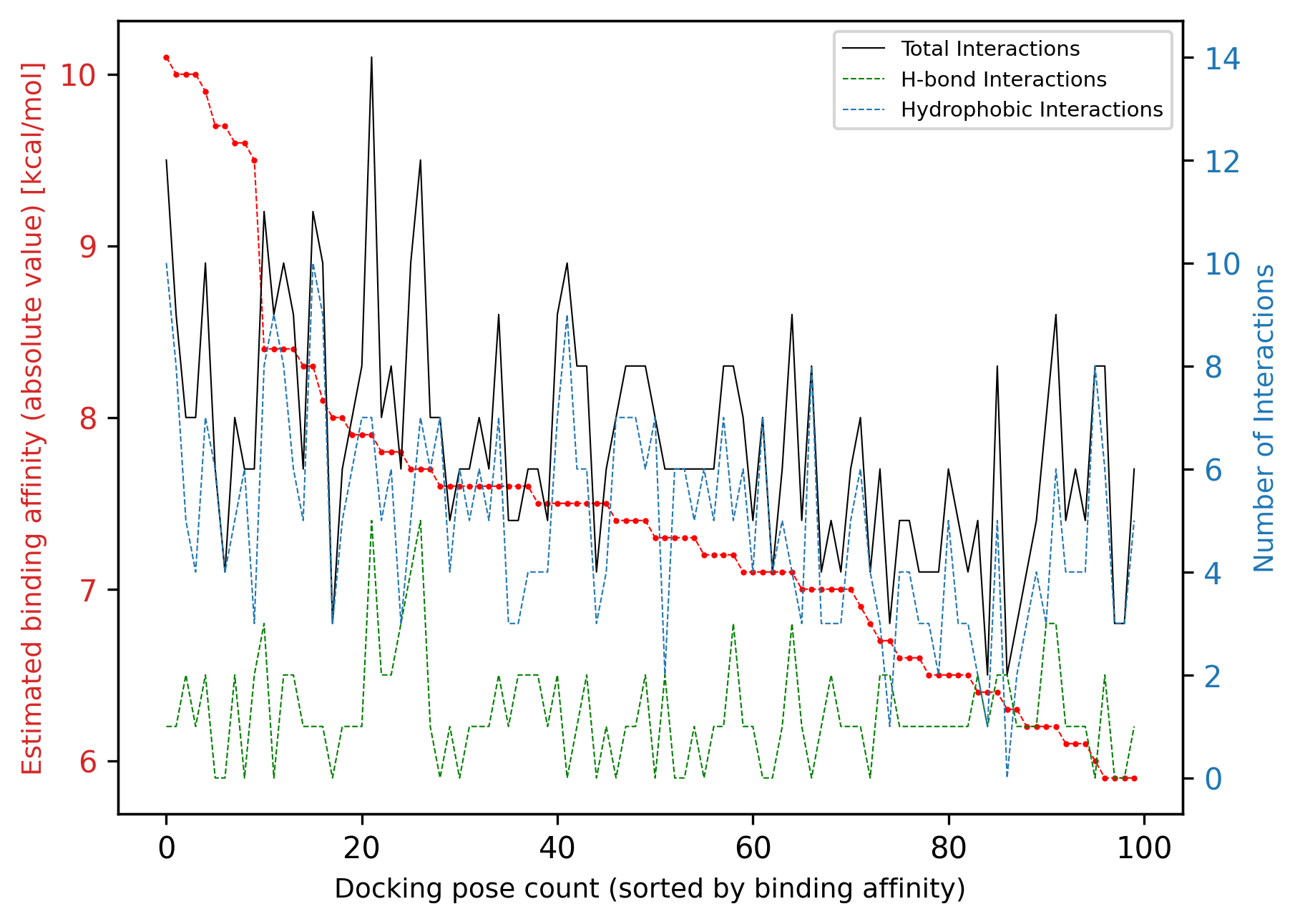
We see that no obvious correlation is visible between the two sets of data; the number of total interactions is weakly correlated with the binding affinity, albeit with several outliers.
Now let’s also analyze the interactions in the docking poses of the input ligand for comparison:
[52]:
project1.Ligand.InteractionAnalysis = InteractionAnalysis(
project1.Docking.pdbqt_filepath_extracted_protein,
project1.Docking.pdb_filepath_extracted_protein,
project1.Protein.residue_number_first,
[project1.Ligand],
project1.Ligand.Docking.master_df,
project1.Specs.InteractionAnalysis,
project1.Specs.OutputPaths.ligand,
)
The results can be viewed in a similar way to the analogs. For example, to view the summary data:
[53]:
project1.Ligand.InteractionAnalysis.results.sort_values(
by="total_num_interactions", ascending=False
)
[53]:
| affinity[kcal/mol] | dist from best mode_rmsd_l.b | dist from best mode_rmsd_u.b | drug_score_total | total_num_interactions | h_bond | hydrophobic | salt_bridge | water_bridge | pi_stacking | pi_cation | halogen | metal | ||
|---|---|---|---|---|---|---|---|---|---|---|---|---|---|---|
| CID | mode | |||||||||||||
| 2426 | 5 | -8.4 | 2.002 | 3.534 | 0.7 | 9 | 2 | 7 | 0 | 0 | 0 | 0 | 0 | 0 |
| 1 | -8.7 | 0.000 | 0.000 | 0.7 | 8 | 2 | 6 | 0 | 0 | 0 | 0 | 0 | 0 | |
| 2 | -8.7 | 1.839 | 2.339 | 0.7 | 6 | 2 | 4 | 0 | 0 | 0 | 0 | 0 | 0 | |
| 3 | -8.7 | 3.811 | 5.375 | 0.7 | 5 | 2 | 3 | 0 | 0 | 0 | 0 | 0 | 0 | |
| 4 | -8.7 | 3.340 | 4.918 | 0.7 | 5 | 2 | 3 | 0 | 0 | 0 | 0 | 0 | 0 |
Again, we see that the pipeline has successfully found analogs that have docking poses with higher number of interactions (up to 12) than those of the input ligand (up to 8).
Visual interaction analysis
Thanks to the nglview helper module, we have additional methods available in the InteractionAnalysis class for visualization of the protein-ligand interactions. For example, we can now view the interactions for all docking poses in an interactive way. By selecting each docking pose from the menu (labeled by their CID and mode-number and sorted by their binding affinities), all the interacting residues are shown. The interactions are visualized with colored lines, for which a color-map is
also provided.
Alternatively, if we are interested in visualization of a certain analog’s interactions, we can use the visualize_analog_interactions method instead, and provide the analog’s CID.
Note: Clicking through different ligands and docking poses works only when you execute this talktorial; it does not work on the website version of the talktorial.
[54]:
project1.InteractionAnalysis.visualize_all_interactions()
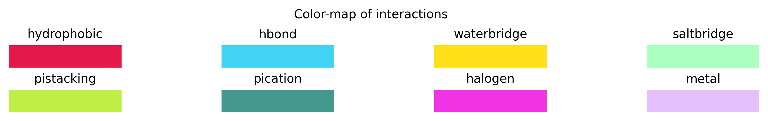
[54]:
Finding poses with specific interactions
We can also search for docking poses displaying a specific set of interactions with specific residues of the protein, using the find_poses_with_specific_interactions method. This returns a list of tuples, where the first tuple element is the CID, and the second element is its corresponding docking pose number in which the specified interaction exists.
We can provide a set of desired interactions to the function, and specify whether we are looking for docking poses that exhibit all or any of these interactions.
For example, since it’s a common interaction in many kinase inhibitors, we can search for the ligands that are involved in hydrogen-bonding with the hinge region of the protein (i.e. residue M793 in EGFR):
[55]:
analog_poses_with_desired_interactions = (
project1.InteractionAnalysis.find_poses_with_specific_interactions(
list_interaction_data=[["h_bond", 793]], all_or_any="any"
)
)
analog_poses_with_desired_interactions
[55]:
[('65997', 2),
('1530', 3),
('11256587', 5),
('62274', 4),
('53462', 2),
('103148', 5)]
Using the visualize_docking_poses_interactions method, we can also visualize the results separately instead of looking for them in the menu of the viewer above. This method takes a list of docking poses (as tuples, where the first elements are the CIDs, and the second elements are the docking pose numbers; i.e. exactly the output format of find_poses_with_specific_interactions) and visualizes them:
[56]:
project1.InteractionAnalysis.visualize_docking_poses_interactions(
list_of_cid_pose_nr_tuples=analog_poses_with_desired_interactions
)

[56]:
Selection of the best analog
At this point, we have carried out all the processes in the pipeline and have gathered all the information in our LeadOptimizationPipeline instance, i.e. project1.
To recap, we have
found the most suitable binding site in the input protein based on the specifications of our project,
gathered a number of analogs to the input ligand and filtered them to choose those with the highest drug-likeness scores, and
calculated several docking poses and corresponding binding affinities for each analog and analyzed their interactions with the protein.
Now we import the class OptimizedLigands, which takes in the whole project, and based on the specifications in the input file, selects the best analog(s).
[57]:
from utils import OptimizedLigands
project1.OptimizedLigands = OptimizedLigands(project=project1)
The class has a __call__ method, which prints out a summary:
[58]:
project1.OptimizedLigands()
Number of docking poses with higher binding affinity than highest binding affinity of ligand: 10
CIDs of analogs corresponding to these docking poses: [‘11292933’, ‘135398510’]
Number of docking poses with higher number of total interactions than highest interacting pose of ligand: 17
CIDs of analogs corresponding to these docking poses: [‘11256587’, ‘62805’, ‘11292933’, ‘214347’, ‘6451164’, ‘103148’, ‘62275’, ‘65997’, ‘57469’]
Number of docking poses with higher affinity and number of total interactions than best corresponding poses of ligand: 3
CIDs of analogs corresponding to these docking poses: [‘11292933’]
CIDs of analogs with higher binding affinity, number of total interactions and drug-likeness score than ligand: [‘11292933’]
CIDs of selected analogs as final output: [‘11292933’]
Comparison between the input ligand and optimized analog:
| Input Ligand | Optimized Analog | |
|---|---|---|
| Drug-Score | 0.7 | 0.77 |
| Highest Binding Affinity | -8.7 | -10.10 |
| Highest Number of Total Interactions | 9.0 | 12.00 |
We can see that the pipeline successfully found an analog superior to the input ligand in all of the three metrics, i.e. calculated drug-likeness, estimated binding affinity, and total number of protein-ligand interactions.
Lastly we can simply visualize the most suited analog(s) found:
[59]:
project1.OptimizedLigands.show_final_output()
| Value | |
|---|---|
| Property | |
 |
|
| name | Gsk163090 |
| iupac_name | 1-[3-[2-[4-(2-methylquinolin-5-yl)piperazin-1-... |
| smiles | CC1=NC2=C(C=C1)C(=CC=C2)N3CCN(CC3)CCC4=CC(=CC=... |
| cid | 11292933 |
| inchi | InChI=1S/C25H29N5O/c1-19-8-9-22-23(27-19)6-3-7... |
| inchikey | ANGUXJDGJCHGOG-UHFFFAOYSA-N |
| mol_weight | 415.541 |
| num_H_acceptors | 4 |
| num_H_donors | 1 |
| logp | 3.44 |
| tpsa | 51.71 |
| num_rot_bonds | 5 |
| saturation | 0.36 |
| drug_score_qed | 0.69 |
| drug_score_lipinski | 1.0 |
| drug_score_custom | 0.77 |
| drug_score_total | 0.77 |
| similarity | 0.2 |
| binding_affinity_best | -10.1 |
| binding_affinity_mean | -9.860000000000001 |
| binding_affinity_std | 0.20736441353327736 |
| docking_poses_dist_rmsd_lb_mean | 1.5622 |
| docking_poses_dist_rmsd_lb_std | 0.888192940751051 |
| docking_poses_dist_rmsd_ub_mean | 2.216 |
| docking_poses_dist_rmsd_ub_std | 1.2926940860079774 |
| average_num_total_interactions | 8.4 |
| average_num_h_bond | 1.2 |
| average_num_hydrophobic | 6.8 |
| average_num_salt_bridge | 0.4 |
| average_num_water_bridge | 0.0 |
| average_num_pi_stacking | 0.0 |
| average_num_pi_cation | 0.0 |
| average_num_halogen | 0.0 |
| average_num_metal | 0.0 |
The final output of the pipeline is thus a certain number (specified in the input specifications) of Ligand objects corresponding to the optimized analogs found:
[60]:
project1.OptimizedLigands.output
# NBVAL_CHECK_OUTPUT
[60]:
[<Ligand CID: 11292933>]
Putting the pieces together: A fully automated pipeline
Now that we have separately demonstrated all the different parts of our pipeline, we will introduce a method —LeadOptimizationPipeline.run — to automatically run the whole pipeline and display the results. It takes in the project name, the filepath of the input data, and the output path, and performs all the necessary processes to generate the final output. It will also print a summary of the intermediate results for each part of the pipeline, so that the process can be followed.
For this demonstration, let’s take the optimized analog we just found and use it as the input ligand to see whether we can do better than our previous optimization results and obtain an even better analog.
We first need to create the corresponding input file. To do so, we can simply open the input file of our project, modify the ligand input value, and save the file as a new input file:
[61]:
new_input_df = pd.read_csv(project1.Specs.RawData.filepath)
new_input_df.head()
# NBVAL_CHECK_OUTPUT
[61]:
| Subject | Property | Value | Description | |
|---|---|---|---|---|
| 0 | Protein | Input Type* | pdb_code | Allowed: 'pdb_code', 'pdb_filepath'. |
| 1 | Protein | Input Value* | 3W32 | Either a valid PDB-code or a local filepath to... |
| 2 | Ligand | Input Type* | smiles | Allowed: 'smiles', 'cid', 'inchi', 'inchikey',... |
| 3 | Ligand | Input Value* | Nc1cc2ncnc(Nc3cccc(Br)c3)c2cc1N | Identifier value corresponding to given input ... |
| 4 | Binding Site | Definition Method | detection | Definition method for the protein binding site... |
[62]:
new_input_df.loc[3, "Value"] = project1.OptimizedLigands.output[0].smiles
new_input_df.head()
# NBVAL_CHECK_OUTPUT
[62]:
| Subject | Property | Value | Description | |
|---|---|---|---|---|
| 0 | Protein | Input Type* | pdb_code | Allowed: 'pdb_code', 'pdb_filepath'. |
| 1 | Protein | Input Value* | 3W32 | Either a valid PDB-code or a local filepath to... |
| 2 | Ligand | Input Type* | smiles | Allowed: 'smiles', 'cid', 'inchi', 'inchikey',... |
| 3 | Ligand | Input Value* | CC1=NC2=C(C=C1)C(=CC=C2)N3CCN(CC3)CCC4=CC(=CC=... | Identifier value corresponding to given input ... |
| 4 | Binding Site | Definition Method | detection | Definition method for the protein binding site... |
[63]:
new_input_df.to_csv(DATA / "PipelineInputData_Project2.csv")
Now let’s run the pipeline again, this time fully automated and with the already optimized ligand as input. Other than printing out a short summary of results in real-time, at the end the function also returns the whole project as a LeadOptimizationPipeline object similar to project1. Thus, by assigning the return value to a variable (here project2), we can later further investigate the information generated by the pipeline in more detail.
Note: We are again using frozen data for the similarity search results and generation of 3D conformations for the analogs to ensure the stability of the pipeline’s results (see here).
[64]:
project2 = LeadOptimizationPipeline.run(
project_name="Project2_EGFR_CID11292933",
input_data_filepath=DATA / "PipelineInputData_Project2.csv",
output_data_root_folder_path=DATA / "Outputs",
frozen_data_filepath=frozen_data_project2.pipeline,
)
Initializing Project: Successful
Project name: Project2_EGFR_CID11292933
Initializing Input/Output: Successful
Input data read from: /Users/sakhawathsumit/Documents/teachopencadd/teachopencadd/talktorials/T018_automated_cadd_pipeline/data/PipelineInputData_Project2.csv
Output folders created at: /Users/sakhawathsumit/Documents/teachopencadd/teachopencadd/talktorials/T018_automated_cadd_pipeline/data/Outputs/Project2_EGFR_CID11292933
Sending GET request to https://files.rcsb.org/download/3W32.pdb to fetch 3W32's pdb file as a string.
Processing Protein: Successful
Structure Title: EGFR KINASE DOMAIN COMPLEXED WITH COMPOUND 20A
Name: EPIDERMAL GROWTH FACTOR RECEPTOR
Chains: [‘A’]
Ligands: [[‘W32’, ‘A1101’, 39], [‘SO4’, ‘A1102’, 5]]
First Residue Number: 701
Last Residue Number: 1017
Number of Residues: 317
Sending GET request to https://files.rcsb.org/download/3W32.pdb to fetch 3W32's pdb file as a string.
Processing Ligand: Successful
| Value | |
|---|---|
| Property | |
|
|
| name | Gsk163090 |
| iupac_name | 1-[3-[2-[4-(2-methylquinolin-5-yl)piperazin-1-... |
| smiles | CC1=NC2=C(C=C1)C(=CC=C2)N3CCN(CC3)CCC4=CC(=CC=... |
| cid | 11292933 |
| inchi | InChI=1S/C25H29N5O/c1-19-8-9-22-23(27-19)6-3-7... |
| inchikey | ANGUXJDGJCHGOG-UHFFFAOYSA-N |
| mol_weight | 415.541 |
| num_H_acceptors | 4 |
| num_H_donors | 1 |
| logp | 3.44 |
| tpsa | 51.71 |
| num_rot_bonds | 5 |
| saturation | 0.36 |
| drug_score_qed | 0.69 |
| drug_score_lipinski | 1.0 |
| drug_score_custom | 0.77 |
| drug_score_total | 0.77 |
Binding Site Detection: Successful
Binding site definition method: DETECTION
Binding site detection method: DOGSITESCORER
Selection method for best binding site: SORTING
Selection criteria for best binding site: [‘lig_cov’, ‘poc_cov’]
Name of selected binding site: P_0_0
Binding site coordinates - center: [15.91, 32.33, 11.03]
Binding site coordinates - size: [24.84, 24.84, 24.84]
[14:36:50] DEPRECATION WARNING: please use MorganGenerator
[14:36:50] DEPRECATION WARNING: please use MorganGenerator
[14:36:50] DEPRECATION WARNING: please use MorganGenerator
[14:36:50] DEPRECATION WARNING: please use MorganGenerator
[14:36:50] DEPRECATION WARNING: please use MorganGenerator
[14:36:50] DEPRECATION WARNING: please use MorganGenerator
[14:36:50] DEPRECATION WARNING: please use MorganGenerator
[14:36:50] DEPRECATION WARNING: please use MorganGenerator
[14:36:50] DEPRECATION WARNING: please use MorganGenerator
[14:36:50] DEPRECATION WARNING: please use MorganGenerator
[14:36:50] DEPRECATION WARNING: please use MorganGenerator
[14:36:50] DEPRECATION WARNING: please use MorganGenerator
[14:36:50] DEPRECATION WARNING: please use MorganGenerator
[14:36:50] DEPRECATION WARNING: please use MorganGenerator
[14:36:50] DEPRECATION WARNING: please use MorganGenerator
[14:36:50] DEPRECATION WARNING: please use MorganGenerator
[14:36:50] DEPRECATION WARNING: please use MorganGenerator
[14:36:50] DEPRECATION WARNING: please use MorganGenerator
[14:36:50] DEPRECATION WARNING: please use MorganGenerator
[14:36:50] DEPRECATION WARNING: please use MorganGenerator
[14:36:50] DEPRECATION WARNING: please use MorganGenerator
[14:36:50] DEPRECATION WARNING: please use MorganGenerator
[14:36:50] DEPRECATION WARNING: please use MorganGenerator
[14:36:50] DEPRECATION WARNING: please use MorganGenerator
[14:36:50] DEPRECATION WARNING: please use MorganGenerator
[14:36:50] DEPRECATION WARNING: please use MorganGenerator
[14:36:50] DEPRECATION WARNING: please use MorganGenerator
[14:36:50] DEPRECATION WARNING: please use MorganGenerator
[14:36:50] DEPRECATION WARNING: please use MorganGenerator
[14:36:50] DEPRECATION WARNING: please use MorganGenerator
[14:36:50] DEPRECATION WARNING: please use MorganGenerator
[14:36:50] DEPRECATION WARNING: please use MorganGenerator
[14:36:50] DEPRECATION WARNING: please use MorganGenerator
[14:36:50] DEPRECATION WARNING: please use MorganGenerator
[14:36:50] DEPRECATION WARNING: please use MorganGenerator
[14:36:50] DEPRECATION WARNING: please use MorganGenerator
[14:36:50] DEPRECATION WARNING: please use MorganGenerator
[14:36:50] DEPRECATION WARNING: please use MorganGenerator
[14:36:50] DEPRECATION WARNING: please use MorganGenerator
[14:36:50] DEPRECATION WARNING: please use MorganGenerator
[14:36:50] DEPRECATION WARNING: please use MorganGenerator
[14:36:50] DEPRECATION WARNING: please use MorganGenerator
[14:36:50] DEPRECATION WARNING: please use MorganGenerator
[14:36:50] DEPRECATION WARNING: please use MorganGenerator
[14:36:50] DEPRECATION WARNING: please use MorganGenerator
[14:36:50] DEPRECATION WARNING: please use MorganGenerator
[14:36:50] DEPRECATION WARNING: please use MorganGenerator
[14:36:50] DEPRECATION WARNING: please use MorganGenerator
[14:36:50] DEPRECATION WARNING: please use MorganGenerator
[14:36:50] DEPRECATION WARNING: please use MorganGenerator
[14:36:50] DEPRECATION WARNING: please use MorganGenerator
[14:36:50] DEPRECATION WARNING: please use MorganGenerator
[14:36:50] DEPRECATION WARNING: please use MorganGenerator
[14:36:50] DEPRECATION WARNING: please use MorganGenerator
[14:36:50] DEPRECATION WARNING: please use MorganGenerator
[14:36:50] DEPRECATION WARNING: please use MorganGenerator
[14:36:50] DEPRECATION WARNING: please use MorganGenerator
[14:36:50] DEPRECATION WARNING: please use MorganGenerator
[14:36:50] DEPRECATION WARNING: please use MorganGenerator
[14:36:50] DEPRECATION WARNING: please use MorganGenerator
[14:36:53] DEPRECATION WARNING: please use MorganGenerator
[14:36:53] DEPRECATION WARNING: please use MorganGenerator
[14:36:55] DEPRECATION WARNING: please use MorganGenerator
[14:36:55] DEPRECATION WARNING: please use MorganGenerator
[14:36:58] DEPRECATION WARNING: please use MorganGenerator
[14:36:58] DEPRECATION WARNING: please use MorganGenerator
[14:37:01] DEPRECATION WARNING: please use MorganGenerator
[14:37:01] DEPRECATION WARNING: please use MorganGenerator
[14:37:03] DEPRECATION WARNING: please use MorganGenerator
[14:37:03] DEPRECATION WARNING: please use MorganGenerator
[14:37:06] DEPRECATION WARNING: please use MorganGenerator
[14:37:06] DEPRECATION WARNING: please use MorganGenerator
[14:37:09] DEPRECATION WARNING: please use MorganGenerator
[14:37:09] DEPRECATION WARNING: please use MorganGenerator
[14:37:11] DEPRECATION WARNING: please use MorganGenerator
[14:37:11] DEPRECATION WARNING: please use MorganGenerator
[14:37:14] DEPRECATION WARNING: please use MorganGenerator
[14:37:14] DEPRECATION WARNING: please use MorganGenerator
[14:37:18] DEPRECATION WARNING: please use MorganGenerator
[14:37:18] DEPRECATION WARNING: please use MorganGenerator
[14:37:21] DEPRECATION WARNING: please use MorganGenerator
[14:37:21] DEPRECATION WARNING: please use MorganGenerator
[14:37:23] DEPRECATION WARNING: please use MorganGenerator
[14:37:23] DEPRECATION WARNING: please use MorganGenerator
[14:37:26] DEPRECATION WARNING: please use MorganGenerator
[14:37:26] DEPRECATION WARNING: please use MorganGenerator
[14:37:28] DEPRECATION WARNING: please use MorganGenerator
[14:37:28] DEPRECATION WARNING: please use MorganGenerator
[14:37:31] DEPRECATION WARNING: please use MorganGenerator
[14:37:31] DEPRECATION WARNING: please use MorganGenerator
[14:37:34] DEPRECATION WARNING: please use MorganGenerator
[14:37:34] DEPRECATION WARNING: please use MorganGenerator
[14:37:36] DEPRECATION WARNING: please use MorganGenerator
[14:37:36] DEPRECATION WARNING: please use MorganGenerator
[14:37:39] DEPRECATION WARNING: please use MorganGenerator
[14:37:39] DEPRECATION WARNING: please use MorganGenerator
[14:37:42] DEPRECATION WARNING: please use MorganGenerator
[14:37:42] DEPRECATION WARNING: please use MorganGenerator
[14:37:45] DEPRECATION WARNING: please use MorganGenerator
[14:37:45] DEPRECATION WARNING: please use MorganGenerator
Ligand Similarity Search: Successful
Search engine: PUBCHEM
Number of fetched analogs with a similarity higher than 70%: 30
Dice-similarity range of fetched analogs: 0.14 - 0.39
CID of analog with the highest Dice-similarity: 60149
Number of selected drug-like analogs: 20
Range of drug-likeness score in selected analogs: 0.71 - 0.92
CID of analog with the highest drug-likeness score: 5761
Docking Experiment: Successful
Highest binding affinity of input ligand: -10.2
Binding affinity range of analogs: -6.3 - -10.8
Number of analog docking poses with higher affinity than ligand: 2
Number of analogs with higher affinity than ligand: 2
CIDs of analogs with higher affinity than ligand: {‘28693’, ‘60149’}
Docking modes
(CID - mode)
Protein-Ligand Interaction Analysis: Successful
Highest number of total interactions in a docking pose of input ligand: 13
Range of total number of interactions in docking poses of analogs: 3 - 13
Correlation plot between binding affinity and number of interactions in docking poses of analogs:
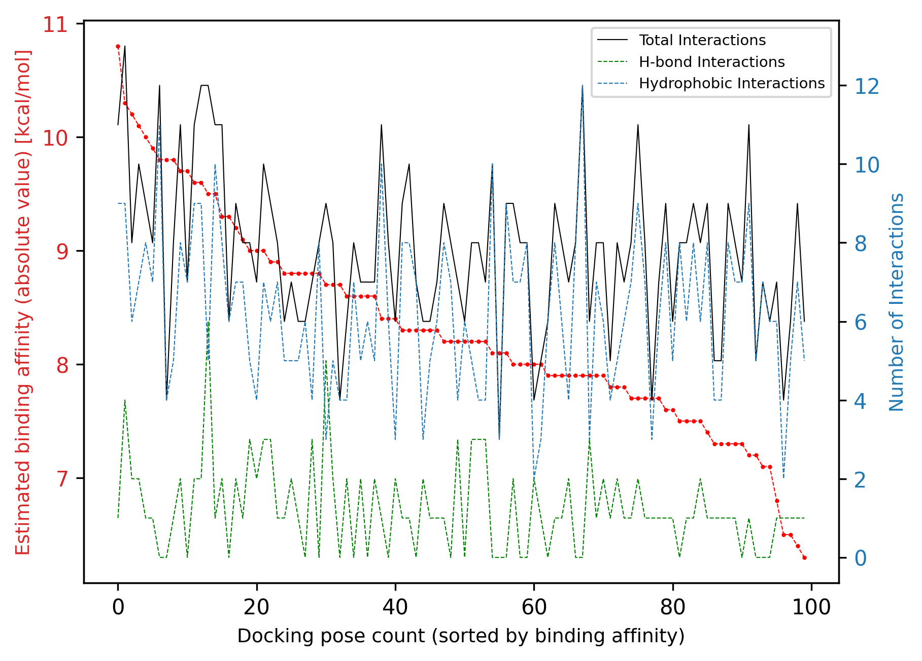

Selecting The Optimized Analog: Successful
Number of docking poses with higher binding affinity than highest binding affinity of ligand: 3
CIDs of analogs corresponding to these docking poses: [‘28693’, ‘60149’]
Number of docking poses with higher number of total interactions than highest interacting pose of ligand: 1
CIDs of analogs corresponding to these docking poses: [‘60149’]
Number of docking poses with higher affinity and number of total interactions than best corresponding poses of ligand: 1
CIDs of analogs corresponding to these docking poses: [‘60149’]
CIDs of analogs with higher binding affinity, number of total interactions and drug-likeness score than ligand: []
CIDs of selected analogs as final output: [‘28693’]
Comparison between the input ligand and optimized analog:
| Input Ligand | Optimized Analog | |
|---|---|---|
| Drug-Score | 0.77 | 0.78 |
| Highest Binding Affinity | -10.20 | -10.80 |
| Highest Number of Total Interactions | 13.00 | 12.00 |
Selected analogs as final output:
| Value | |
|---|---|
| Property | |
 |
|
| name | Metergoline |
| iupac_name | benzyl N-[[(6aR,9S,10aR)-4,7-dimethyl-6,6a,8,9... |
| smiles | CN1CC(CC2C1CC3=CN(C4=CC=CC2=C34)C)CNC(=O)OCC5=... |
| cid | 28693 |
| inchi | InChI=1S/C25H29N3O2/c1-27-14-18(13-26-25(29)30... |
| inchikey | WZHJKEUHNJHDLS-QTGUNEKASA-N |
| mol_weight | 403.526 |
| num_H_acceptors | 4 |
| num_H_donors | 1 |
| logp | 4.06 |
| tpsa | 46.5 |
| num_rot_bonds | 4 |
| saturation | 0.4 |
| drug_score_qed | 0.71 |
| drug_score_lipinski | 1.0 |
| drug_score_custom | 0.78 |
| drug_score_total | 0.78 |
| similarity | 0.23 |
| binding_affinity_best | -10.8 |
| binding_affinity_mean | -10.079999999999998 |
| binding_affinity_std | 0.42071367935925263 |
| docking_poses_dist_rmsd_lb_mean | 2.086 |
| docking_poses_dist_rmsd_lb_std | 1.4826484748584203 |
| docking_poses_dist_rmsd_ub_mean | 4.6972000000000005 |
| docking_poses_dist_rmsd_ub_std | 4.087722006203456 |
| average_num_total_interactions | 9.0 |
| average_num_h_bond | 0.8 |
| average_num_hydrophobic | 7.6 |
| average_num_salt_bridge | 0.6 |
| average_num_water_bridge | 0.0 |
| average_num_pi_stacking | 0.0 |
| average_num_pi_cation | 0.0 |
| average_num_halogen | 0.0 |
| average_num_metal | 0.0 |

Pipeline Completed: Successful
As you can see, the pipeline was again successful in finding an analog (CID: 28693) to the optimized analog of project1 (CID: 11292933) with a higher estimated binding affinity (-10.8 kcal/mol versus -10.2 kcal/mol). The pipeline was even able to find another analog (CID: 60149) with both a higher binding affinity (but not as high as that of compound 28693) and a higher number of interactions, but since in the input specifications we have prioritized binding affinity over the number of
interactions, the OptimizedLigands class still selected the compound 28693.
Nevertheless, we can still have a look at the analog(s) with both higher affinity and number of interactions than the input ligand (i.e. compound 60149 in this case):
[65]:
project2.OptimizedLigands.higher_affinity_and_interacting_analogs
[65]:
[<Ligand CID: 60149>]
[66]:
project2.OptimizedLigands.higher_affinity_and_interacting_analogs[0]()
[66]:
| Value | |
|---|---|
| Property | |
 |
|
| name | Sertindole |
| iupac_name | 1-[2-[4-[5-chloro-1-(4-fluorophenyl)indol-3-yl... |
| smiles | C1CN(CCC1C2=CN(C3=C2C=C(C=C3)Cl)C4=CC=C(C=C4)F... |
| cid | 60149 |
| inchi | InChI=1S/C24H26ClFN4O/c25-18-1-6-23-21(15-18)2... |
| inchikey | GZKLJWGUPQBVJQ-UHFFFAOYSA-N |
| mol_weight | 440.95 |
| num_H_acceptors | 3 |
| num_H_donors | 1 |
| logp | 4.63 |
| tpsa | 40.51 |
| num_rot_bonds | 5 |
| saturation | 0.38 |
| drug_score_qed | 0.63 |
| drug_score_lipinski | 1.0 |
| drug_score_custom | 0.71 |
| drug_score_total | 0.72 |
| similarity | 0.39 |
| binding_affinity_best | -10.3 |
| binding_affinity_mean | -9.74 |
| binding_affinity_std | 0.5319774431308155 |
| docking_poses_dist_rmsd_lb_mean | 2.5082 |
| docking_poses_dist_rmsd_lb_std | 1.7358681401535083 |
| docking_poses_dist_rmsd_ub_mean | 4.157 |
| docking_poses_dist_rmsd_ub_std | 3.1173451846082103 |
| average_num_total_interactions | 8.6 |
| average_num_h_bond | 1.6 |
| average_num_hydrophobic | 6.6 |
| average_num_salt_bridge | 0.2 |
| average_num_water_bridge | 0.0 |
| average_num_pi_stacking | 0.0 |
| average_num_pi_cation | 0.2 |
| average_num_halogen | 0.0 |
| average_num_metal | 0.0 |
Just like project1, the final output of the pipeline is also directly accesible as a Ligand object:
[67]:
project2.OptimizedLigands.output
# NBVAL_CHECK_OUTPUT
[67]:
[<Ligand CID: 28693>]
Discussion
In this talktorial, we successfully implemented a fully-automated virtual screening pipeline targeted at hit-expansion and lead-optimization phases of a drug discovery project. The pipeline is designed to take in a target protein structure and a promising ligand (i.e. initial hit/lead compound), and carry out the necessary processes according to the user specifications in order to suggest an optimized analog of the input ligand, in terms of estimated binding affinity, number and type of protein—ligand interactions, and drug-likeness.
Click here for a more detailed summary of the pipeline’s architecture and processes.
As input, the pipeline accepts a single CSV file, specifying a protein structure, a ligand, and various other project-specific settings for the different processes of the pipeline, e.g. criteria for the selection of the most suited binding pocket, and for finding and selecting analogs, as well as docking specifications, or desired protein—ligand interactions to look for.
The code is compartmentalized into eight main classes — each of which being responsible for a specific task in the pipeline (Figure 8) — as follows:
``Specs``: reads and processes the input data for further use in the pipeline, and creates output paths to store all the data generated throughout the whole process.
``Protein``: uses the input protein data to create a
Proteinobject that provides extended information (in form of attributes) on the protein, as well as various methods to manipulate, analyze and visualize the protein data.``Ligand``: creates a
Ligandobject from the input ligand data, with extended attributes and methods similar to theProteinobject.``BindingSiteDetection``: provides methods to automatically perform all the necessary processes for the selection of the best protein binding site according to the input specifications. For our demonstrations in this talktorial, we used the DoGSiteScorer functionality of the ProteinsPlus webserver as our binding site detection method.
``LigandSimilaritySearch``: contains all required functionalities to automatically execute a ligand similarity search to find suitable analogs according to the input specifications. In this talktorial, the similarity search was done using the PubChem web-services via the provided API backend. This class is also responsible for filtering the analogs based on several calculated drug-likeness scores.
``Docking``: is responsible for carrying out the docking calculations and analyzing and visualizing the results. We used the Smina program for the docking experiments, and the
`NGLview<https://doi.org/10.1093/bioinformatics/btx789>`__ widget to visualize the docking poses.``InteractionAnalysis``: consists of methods to analyze and visualize the protein—ligand interactions in the docking poses generated by
Docking. The analysis was done with the help of the`PLIP<https://github.com/pharmai/plip>`__ package - a Python package for the Protein—Ligand Interaction Profiler (PLIP), and the interactions were visualized with the NGLview widget.``OptimizedLigands``: analyzes the whole data generated by the pipeline in order to select the best analogs based on criteria specified in the input settings.
Moreover, a container class called ``LeadOptimizationPipeline`` is defined, which provides a method run that puts the whole pipeline together and automatically executes a given project to completion, merely by providing its input specification file. In this way, all the project’s data and outputs generated by the pipeline are contained within a single object, along with all implemented functionalities, ready for further analysis or use in other programs.
We first demonstrated the pipeline in a step-by-step fashion, using EGFR (PDB code: 3W32) as the target protein, and a promising inhibitor with the ChEMBL compound-ID CHEMBL328216 (Figure 9). After performing all the necessary processes according to the input specifications, the pipeline was able to suggest an analog of the provided ligand with optimized features in terms of estimated binding affinity (-10.2 vs. -8.8 kcal/mol), number of protein—ligand interactions (11 vs. 8) and calculated drug-likeness (77 vs 70%).
Subsequently, we also showcased the pipeline’s ability to run fully automatically. For this purpose, we tried to re-optimize the suggested analog, by keeping the same project specifications and only replacing the input ligand with the optimized analog found in the first run. This second run yielded yet another analog with an improved estimated binding affinity (-10.8 vs -10.2 kcal/mol).
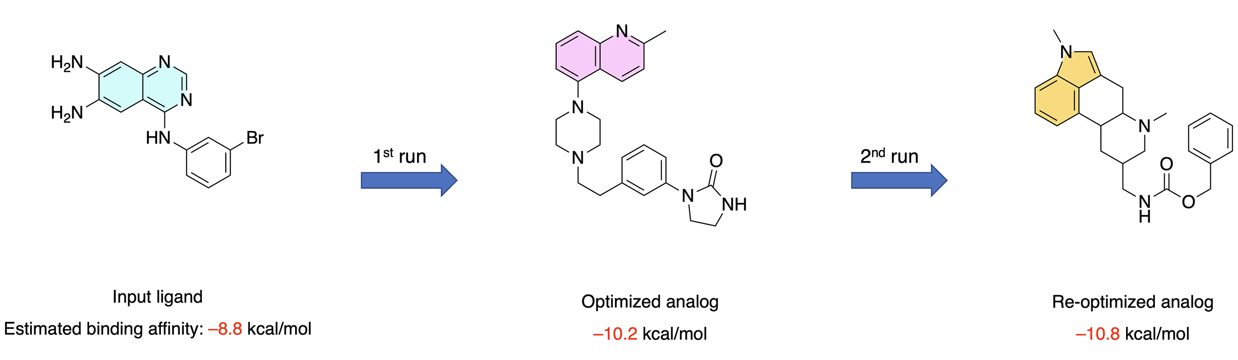
Figure 9. Results of the pipeline’s performance in the demonstrated examples. Starting with a ligand with an estimated binding affinity of -8.8 kcal/mol, the pipeline was able to suggest an analog with an improved estimated affinity of -10.2 kcal/mol. Subjecting this optimized ligand to the same process resulted in another analog with an estimated binding affinity of -10.8 kcal/mol.
However, the results of the pipeline are not fully deterministic by default. This is due to the interaction of the pipeline with online databases that are being constantly updated (i.e the PubChem database used for ligand similarity search) and calculations that have unavoidable randomized components (i.e. generating initial conformations for docking experiments using the OpenBabel package). Thus, to maintain the stability of this talktorial’s results, we have circumvented this issue by freezing the outputs of the mentioned processes. Of course, this can be easily undone by modifying a single variable, so that you can easily use the pipeline for your own project.
The pipeline’s code is specifically structured in such a way that it will be easy to digest, maintain and expand. For each functionality of the pipeline, a separate class was created using several helper modules that can be easily adopted and built upon for various situations and needs. As the pipeline also provides other options outside the scope of this talktorial, we have provided a Supplementary Information section that demonstrates the use of these helper modules and showcases the possibilities of the pipeline in more detail.
Quiz
Conceptual Questions:
Describe the processes involved in the hit-to-lead and lead optimization phases of a drug design pipeline. How are these processes implemented in the virtual pipeline described in this talktorial?
Describe the important facets of binding site definition in a general virtual screening pipeline. What options are available for binding site definition and selection in this pipeline?
How can we use the pipeline to find analogs with a higher selectivity for the target protein?
Which parts of the pipeline are not fully deterministic and why? How have we circumvented this in the talktorial?
Practical Tasks:
In order to prevent the talktorial from being too lengthy, we only demonstrated a subset of the possibilities and information that the pipeline offers. Execute the pipeline by creating another
LeadOptimizationPipelineinstance (ideally with a different protein and ligand), and explore its other options by looking up the attributes and methods that the main classes of the pipeline have to offer.Generate your own input CSV files, each time choosing a different set of specifications, and compare the results. Can you find a set of specifications that perform considerably better than the others?
Try to implement a loop, where the final output of a pipeline is re-entered as the input for a new pipeline (i.e. try to optimize your initial input ligand through several runs, same as we did for the demonstration of the
LeadOptimizationPipeline.runmethod). After how many cycles does the pipeline reach a plateau where results no longer improve?
Supplementary information
Here we will demonstrate the functions of each helper module used in the pipeline, to provide a better understanding of the inner workings of the code. These modules supply the fundamental functionalities that the main classes of the pipeline rely on, and can be easily adopted for use in other bioinformatics programs.
Note: Some cells use variables defined in an early cell. Therefore, in order for all cells to work properly, you have to run them sequentially.
Demonstration of the io helper module
This module is mainly used in the class Specs of the pipeline, and contains the basic functions required for handling the input and output data, e.g. creating a pandas dataframe from the input CSV file, extracting specific information from the dataframe, or creating folders for storing the output data.
[68]:
from utils import Consts
from utils.helpers import io
The input CSV file can be easily imported as a Pandas DataFrame via the create_dataframe_from_csv_input_file function, by specifying the corresponding filepath, the name of the columns to be used as index columns for the dataframe, and the name of the other columns we want to keep.
Note: While we can explicitly use the name of the columns (i.e. "Subject", "Property" and "Value") for inputting list_of_index_column_names and list_of_column_names_to_keep parameters, we will use the respective constants stored in the Consts class. In this way, if the column names in the input file are changed in the future, they only need to be corrected in the Consts class and nowhere else in the code.
[69]:
example_input_df = io.create_dataframe_from_csv_input_file(
input_data_filepath=DATA / f"PipelineInputData_Project1.csv",
list_of_index_column_names=[
Consts.DataFrame.ColumnNames.SUBJECT.value,
Consts.DataFrame.ColumnNames.PROPERTY.value,
],
list_of_columns_to_keep=[Consts.DataFrame.ColumnNames.VALUE.value],
)
example_input_df
[69]:
| Value | ||
|---|---|---|
| Subject | Property | |
| Protein | Input Type* | pdb_code |
| Input Value* | 3W32 | |
| Ligand | Input Type* | smiles |
| Input Value* | Nc1cc2ncnc(Nc3cccc(Br)c3)c2cc1N | |
| Binding Site | Definition Method | detection |
| Coordinates | NaN | |
| Ligand | NaN | |
| Detection Method | dogsitescorer | |
| Protein Chain-ID | NaN | |
| Protein Ligand-ID | NaN | |
| Selection Method | sorting | |
| Selection Criteria | lig_cov, poc_cov | |
| Ligand Similarity Search | Search Engine | pubchem |
| Minumum Similarity [%] | 70 | |
| Maximum Number of Results | 30 | |
| Maximum Number of Most Drug-Like Analogs to Continue With | 20 | |
| Docking | Program | smina |
| Number of Docking Poses per Ligand | 5 | |
| Exhaustiveness | 10 | |
| Random Seed | 1111 | |
| Interaction Analysis | Program | plip |
| Optimized Ligand | Number of Results | 1 |
| Selection Method | sorting | |
| Selection Criteria | affinity, total_num_interactions, drug_score_t... |
Moreover, we can also extract all the data corresponding to a specific Subject, using the copy_series_from_dataframe function and specifying the main dataframe and the name of the index-level and column that we want to extract. For example, to extract the binding site specification data:
[70]:
example_input_protein_data = io.copy_series_from_dataframe(
input_df=example_input_df,
index_name=Consts.DataFrame.SubjectNames.BINDING_SITE.value,
column_name=Consts.DataFrame.ColumnNames.VALUE.value,
)
example_input_protein_data
[70]:
Property
Definition Method detection
Coordinates NaN
Ligand NaN
Detection Method dogsitescorer
Protein Chain-ID NaN
Protein Ligand-ID NaN
Selection Method sorting
Selection Criteria lig_cov, poc_cov
Name: Value, dtype: object
For storing the output data we will also need the create_folder function, which can create a folder (and all its necessary parent folders) with a given name at a given path. The function then returns the full path of the created folder.
We now create a folder named Examples under our main DATA folder, which we will use to store the files created in this section:
[71]:
example_output_path = io.create_folder(folder_name="Examples", folder_path=DATA / "Outputs")
example_output_path
[71]:
PosixPath('/Users/sakhawathsumit/Documents/teachopencadd/teachopencadd/talktorials/T018_automated_cadd_pipeline/data/Outputs/Examples')
Demonstration of the pdb helper module
This module contains the necessary functions for handling protein data and processing PDB files, e.g. downloading PDB files, reading and extracting useful data, and extracting a certain molecule. It is created using the pypdb and biopandas packages, and is primarily used in the pipeline classes Protein and Docking.
[72]:
from utils.helpers import pdb
We can use the fetch_and_save_pdb_file function to download a protein’s PDB file using its PDB-code. The function also takes in an output filepath and returns the full path of the downloaded file.
Let’s download the structure for the EGFR protein, with the PDB-code 3W32:
[73]:
example_downloaded_protein_filepath = pdb.fetch_and_save_pdb_file(
pdb_code="3w32", output_filepath=example_output_path / "3W32"
)
example_downloaded_protein_filepath
Sending GET request to https://files.rcsb.org/download/3w32.pdb to fetch 3w32's pdb file as a string.
[73]:
PosixPath('/Users/sakhawathsumit/Documents/teachopencadd/teachopencadd/talktorials/T018_automated_cadd_pipeline/data/Outputs/Examples/3W32.pdb')
The PDB file is now downloaded on the disk. The content of the PDB file can now be obtained as follows (since the complete file is very long, here we only show the first 800 characters):
[74]:
example_pdb_file_content_1 = pdb.read_pdb_file_content(
input_type="pdb_filepath", input_value=example_downloaded_protein_filepath
)
example_pdb_file_content_1[:800]
[74]:
'HEADER TRANSFERASE/TRANSFERASE INHIBITOR 07-DEC-12 3W32 \nTITLE EGFR KINASE DOMAIN COMPLEXED WITH COMPOUND 20A \nCOMPND MOL_ID: 1; \nCOMPND 2 MOLECULE: EPIDERMAL GROWTH FACTOR RECEPTOR; \nCOMPND 3 CHAIN: A; \nCOMPND 4 FRAGMENT: KINASE DOMAIN, UNP RESIDUES 696-1022; \nCOMPND 5 SYNONYM: PROTO-ONCOGENE C-ERBB-1, RECEPTOR TYROSINE-PROTEIN KINASE \nCOMPND 6 ERBB-1; \nCOMPND 7 EC: 2.7.10.1; \nCOMPND 8 ENGINEERED: YES '
Note that, alternatively we can also set the parameter input_type to "pdb_code" and enter a valid PDB-code as the input_value to directly fetch and read the file contents of a protein PDB file from the PDB webserver. However, in that case, the PDB file itself would not be saved on the disk:
[75]:
example_pdb_file_content_2 = pdb.read_pdb_file_content(input_type="pdb_code", input_value="3w32")
example_pdb_file_content_2[:800]
Sending GET request to https://files.rcsb.org/download/3w32.pdb to fetch 3w32's pdb file as a string.
[75]:
'HEADER TRANSFERASE/TRANSFERASE INHIBITOR 07-DEC-12 3W32 \nTITLE EGFR KINASE DOMAIN COMPLEXED WITH COMPOUND 20A \nCOMPND MOL_ID: 1; \nCOMPND 2 MOLECULE: EPIDERMAL GROWTH FACTOR RECEPTOR; \nCOMPND 3 CHAIN: A; \nCOMPND 4 FRAGMENT: KINASE DOMAIN, UNP RESIDUES 696-1022; \nCOMPND 5 SYNONYM: PROTO-ONCOGENE C-ERBB-1, RECEPTOR TYROSINE-PROTEIN KINASE \nCOMPND 6 ERBB-1; \nCOMPND 7 EC: 2.7.10.1; \nCOMPND 8 ENGINEERED: YES '
The PDB file content can then be used to extract some useful information on the protein, with the help of the function extract_info_from_pdb_file_content:
[76]:
example_pdb_info_1 = pdb.extract_info_from_pdb_file_content(
pdb_file_text_content=example_pdb_file_content_1
)
example_pdb_info_1
[76]:
{'Structure Title': 'EGFR KINASE DOMAIN COMPLEXED WITH COMPOUND 20A',
'Name': 'EPIDERMAL GROWTH FACTOR RECEPTOR',
'Chains': ['A'],
'Ligands': [['W32', 'A1101', 39], ['SO4', 'A1102', 5]]}
The provided data are:
Title of the PDB structure
Name of the protein
IDs of available chains in the protein structure
Information on each co-crystallized ligand, consisting of ligand-ID, location of the ligand in the protein structure (chain-ID followed by residue number), and number of heavy atoms comprising the ligand.
Another example without storing the PDB file contents (using another PDB-code):
[77]:
example_pdb_info_2 = pdb.extract_info_from_pdb_file_content(
pdb_file_text_content=pdb.read_pdb_file_content(input_type="pdb_code", input_value="5gty")
)
example_pdb_info_2
Sending GET request to https://files.rcsb.org/download/5gty.pdb to fetch 5gty's pdb file as a string.
[77]:
{'Structure Title': 'CRYSTAL STRUCTURE OF EGFR 696-1022 T790M IN COMPLEX WITH LXX-6-26',
'Name': 'EPIDERMAL GROWTH FACTOR RECEPTOR',
'Chains': ['A'],
'Ligands': [['816', 'A1101', 36],
['816', 'B1101', 36],
['816', 'D1101', 36],
['816', 'E1101', 36],
['816', 'F1101', 36],
['816', 'G1101', 36],
['EDO', 'G1102', 4],
['816', 'H1101', 36],
['EDO', 'H1102', 4],
['EDO', 'H1103', 4],
['EDO', 'H1104', 4],
['816', 'C1101', 36]]}
The load_pdb_file_as_dataframe function can also be used to access a set of different more detailed data on the PDB file. The function returns a dictionary where each value is a Pandas DataFrame:
[78]:
example_pdb_dataframe = pdb.load_pdb_file_as_dataframe(
pdb_file_text_content=example_pdb_file_content_1
)
example_pdb_dataframe.keys()
[78]:
dict_keys(['ATOM', 'HETATM', 'ANISOU', 'OTHERS'])
For example, all the information regarding the atoms in the protein can be accessed via the ATOM key. This data was used in the pipeline, for example, to extract the range of residue numbers of the protein.
[79]:
example_pdb_dataframe["ATOM"].head()
[79]:
| record_name | atom_number | blank_1 | atom_name | alt_loc | residue_name | blank_2 | chain_id | residue_number | insertion | ... | x_coord | y_coord | z_coord | occupancy | b_factor | blank_4 | segment_id | element_symbol | charge | line_idx | |
|---|---|---|---|---|---|---|---|---|---|---|---|---|---|---|---|---|---|---|---|---|---|
| 0 | ATOM | 1 | N | GLN | A | 701 | ... | -0.023 | 33.326 | -4.411 | 1.0 | 47.95 | N | NaN | 426 | ||||||
| 1 | ATOM | 2 | CA | GLN | A | 701 | ... | -0.291 | 31.978 | -3.835 | 1.0 | 50.95 | C | NaN | 428 | ||||||
| 2 | ATOM | 3 | C | GLN | A | 701 | ... | 0.946 | 31.062 | -3.957 | 1.0 | 47.20 | C | NaN | 430 | ||||||
| 3 | ATOM | 4 | O | GLN | A | 701 | ... | 0.876 | 29.863 | -3.659 | 1.0 | 47.25 | O | NaN | 432 | ||||||
| 4 | ATOM | 5 | CB | GLN | A | 701 | ... | -1.501 | 31.341 | -4.517 | 1.0 | 64.85 | C | NaN | 434 |
5 rows × 21 columns
Lastly, we can use the function extract_molecule_from_pdb_file to extract a certain molecule from a multi-entry PDB file, such as one containing a protein—ligand complex. This will return an MDAnalysis.core.groups.AtomGroup object from the opencadd package, but more importantly, the function will also save the extracted molecule in a new PDB file in a given path. We will later need the PDB file of the extracted protein for performing docking
calculations.
To extract the protein from the PDB file, we set the parameter molecule_name to “protein”, and provide the filepaths:
[80]:
example_extracted_protein = pdb.extract_molecule_from_pdb_file(
molecule_name="protein",
input_filepath=example_downloaded_protein_filepath,
output_filepath=example_output_path / "extracted_protein.pdb",
)
example_extracted_protein
[80]:
<AtomGroup with 2545 atoms>
Alternatively, to extract a certain ligand, we have to provide its ID (in this structure, the ID of the co-crystallized ligand is W32):
[81]:
example_extracted_ligand = pdb.extract_molecule_from_pdb_file(
molecule_name="W32",
input_filepath=example_downloaded_protein_filepath,
output_filepath=example_output_path / "extracted_ligand.pdb",
)
example_extracted_ligand
[81]:
<AtomGroup with 39 atoms>
Demonstration of the pubchem helper module
This module enables us to communicate with the PubChem database via their PUG-REST API service. It can be used to obtain information on ligands, such as identifiers (e.g. IUPAC name, SMILES, CID), physiochemical properties, textual descriptions etc. These functionalities were used in the class Ligand of the pipeline. Moreover, it allows us to perform similarity searches on a given ligand,
which was used in the class LigandSimilaritySearch.
[82]:
from utils.helpers import pubchem
The convert_compound_identifier function can be used to get a specific compound’s identifier by providing another identifier.
For example, obtaining the SMILES of a compound (here Gefitinib; an EGFR inhibitor) by providing its name:
[83]:
pubchem.convert_compound_identifier(
input_id_type="name", input_id_value="gefitinib", output_id_type="smiles"
)
[83]:
'COC1=C(C=C2C(=C1)N=CN=C2NC3=CC(=C(C=C3)F)Cl)OCCCN4CCOCC4'
Or retrieving its IUPAC name:
[84]:
pubchem.convert_compound_identifier(
input_id_type="name", input_id_value="gefitinib", output_id_type="iupac_name"
)
[84]:
'N-(3-chloro-4-fluorophenyl)-7-methoxy-6-(3-morpholin-4-ylpropoxy)quinazolin-4-amine'
Or retrieving its name using its SMILES:
[85]:
pubchem.convert_compound_identifier(
input_id_type="smiles",
input_id_value="COC1=C(C=C2C(=C1)N=CN=C2NC3=CC(=C(C=C3)F)Cl)OCCCN4CCOCC4",
output_id_type="name",
)
[85]:
'Gefitinib'
Or retrieving its CID using its name:
[86]:
pubchem.convert_compound_identifier(
input_id_type="name", input_id_value="gefitinib", output_id_type="cid"
)
[86]:
'123631'
Using the get_compound_record function, all available records on the molecule is returned as a dictionary:
[87]:
example_compound_records = pubchem.get_compound_record(
input_id_type="name", input_id_value="gefitinib"
)
The available keys and corresponding values in the dictionary are:
id: dictionary containing the identifiers (e.g. CID) of the compound.atoms: dictionary containing information on the number and type of atoms in the compound.bonds: dictionary describing the connectivities (i.e. bonding partners and corresponding bond orders) of each atomcoords: list of dictionaries containing coordinates of various conformers of the compoundscharge: total charge of the compoundprops: list of dictionaries containing several identifiers (e.g. IUPAC name) and physiochemical properties of the compound (e.g. number of hydrogen bond donors and acceptors, number of rotatable bonds, fingerprints etc.)count: dictionary containing several counts for the compound, such as heavy atoms, chiral atoms etc.
[88]:
example_compound_records.keys()
[88]:
dict_keys(['id', 'atoms', 'bonds', 'coords', 'charge', 'props', 'count'])
As an example, we access the props key (only showing the first 3 entries):
[89]:
example_compound_records["props"][:3]
[89]:
[{'urn': {'label': 'Compound',
'name': 'Canonicalized',
'datatype': 5,
'release': '2025.09.15'},
'value': {'ival': 1}},
{'urn': {'label': 'Compound Complexity',
'datatype': 7,
'implementation': 'E_COMPLEXITY',
'version': '3.4.8.24',
'software': 'Cactvs',
'source': 'Xemistry GmbH',
'release': '2025.09.15'},
'value': {'fval': 545}},
{'urn': {'label': 'Count',
'name': 'Hydrogen Bond Acceptor',
'datatype': 5,
'implementation': 'E_NHACCEPTORS',
'version': '3.4.8.24',
'software': 'Cactvs',
'source': 'Xemistry GmbH',
'release': '2025.09.15'},
'value': {'ival': 8}}]
The get_description_from_smiles function provides a textual description of the compound. However, it is not available for every compound. If the parameter printout is set to False, the function will return a dictionary containing the descriptions, sources, and other information. By setting it to True, only the description part will be printed out.
For example, using the SMILES of Gefitinib:
[90]:
pubchem.get_description_from_smiles(
smiles="COC1=C(C=C2C(=C1)N=CN=C2NC3=CC(=C(C=C3)F)Cl)OCCCN4CCOCC4", printout=True
)
Name: Gefitinib
CID: 123631
Gefitinib is a member of the class of quinazolines that is quinazoline which is substituted by a (3-chloro-4-fluorophenyl)nitrilo group, 3-(morpholin-4-yl)propoxy group and a methoxy group at positions 4,6 and 7, respectively. An EGFR kinase inhibitor used for the treatment of non-small cell lung cancer. It has a role as an antineoplastic agent and an epidermal growth factor receptor antagonist. It is an aromatic ether, a member of quinazolines, a member of morpholines, a secondary amino compound, a tertiary amino compound, a member of monochlorobenzenes and a member of monofluorobenzenes.
Source: ChEBI, https://www.ebi.ac.uk/chebi/searchId.do?chebiId=CHEBI:49668
The similarity_search function performs a similarity search on a given compound by providing its SMILES. The min_similarity parameter defines the minimum similarity percent to be considered, while the max_num_results parameter limits the number of results to be fetched from the PubChem server. By default, the results are returned in a json format, which is transformed into a list of dictionaries. However, the return format can also be changed using the optional
output_data_file parameter.
Let’s search for some analogs of Gefitinib:
[91]:
example_analogs = pubchem.similarity_search(
smiles="COC1=C(C=C2C(=C1)N=CN=C2NC3=CC(=C(C=C3)F)Cl)OCCCN4CCOCC4",
min_similarity=70,
max_num_results=5,
)
example_analogs
[91]:
[{'CID': 4680,
'ConnectivitySMILES': 'COC1=C(C=C(C=C1)CC2=NC=CC3=CC(=C(C=C32)OC)OC)OC'},
{'CID': 2092,
'ConnectivitySMILES': 'CN(CCCNC(=O)C1CCCO1)C2=NC3=CC(=C(C=C3C(=N2)N)OC)OC'},
{'CID': 2247,
'ConnectivitySMILES': 'COC1=CC=C(C=C1)CCN2CCC(CC2)NC3=NC4=CC=CC=C4N3CC5=CC=C(C=C5)F'},
{'CID': 68546,
'ConnectivitySMILES': 'COC1=C(C=C2C(=C1)C(=NC(=N2)N3CCN(CC3)C(=O)C4=CC=CO4)N)OC.Cl'},
{'CID': 176870,
'ConnectivitySMILES': 'COCCOC1=C(C=C2C(=C1)C(=NC=N2)NC3=CC=CC(=C3)C#C)OCCOC'}]
We can, for example, get their names as well:
[92]:
for analog in example_analogs:
analog["Name"] = pubchem.convert_compound_identifier(
input_id_type="smiles",
input_id_value=analog["ConnectivitySMILES"], # analog["CanonicalSMILES"]
output_id_type="name",
)
example_analogs
[92]:
[{'CID': 4680,
'ConnectivitySMILES': 'COC1=C(C=C(C=C1)CC2=NC=CC3=CC(=C(C=C32)OC)OC)OC',
'Name': 'Papaverine'},
{'CID': 2092,
'ConnectivitySMILES': 'CN(CCCNC(=O)C1CCCO1)C2=NC3=CC(=C(C=C3C(=N2)N)OC)OC',
'Name': 'Alfuzosin'},
{'CID': 2247,
'ConnectivitySMILES': 'COC1=CC=C(C=C1)CCN2CCC(CC2)NC3=NC4=CC=CC=C4N3CC5=CC=C(C=C5)F',
'Name': 'Astemizole'},
{'CID': 68546,
'ConnectivitySMILES': 'COC1=C(C=C2C(=C1)C(=NC(=N2)N3CCN(CC3)C(=O)C4=CC=CO4)N)OC.Cl',
'Name': 'Prazosin Hydrochloride'},
{'CID': 176870,
'ConnectivitySMILES': 'COCCOC1=C(C=C2C(=C1)C(=NC=N2)NC3=CC=CC(=C3)C#C)OCCOC',
'Name': 'Erlotinib'}]
Demonstration of the rdkit helper module
This module uses the RDKit package to implement some useful functionalities for processing ligand data, such as visualization, calculation of physiochemical properties and descriptors, and measuring similarity between compounds using different metrics. These functions are mostly used in the Ligand class of the pipeline.
[93]:
from utils.helpers import rdkit
To use any other function in the rdkit module, we first have to generate an rdkit.Chem.rdchem.Mol molecule object using the create_molecule_object function. This function accepts different identifiers as input, such as SMILES, SMARTS, or even PDB files.
Let’s create an object for Gefitinib from its SMILES:
[94]:
example_mol_obj = rdkit.create_molecule_object(
input_type="smiles",
input_value="COC1=C(C=C2C(=C1)N=CN=C2NC3=CC(=C(C=C3)F)Cl)OCCCN4CCOCC4",
)
type(example_mol_obj)
[94]:
rdkit.Chem.rdchem.Mol
The rdkit.Chem.rdchem.Mol objects can be called directly, which simply visualizes the molecule:
[95]:
example_mol_obj
[95]:
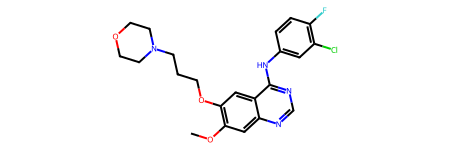
The object itself has several methods and attributes we can make use of; for example, we can now obtain the number of atoms in the molecule:
[96]:
example_mol_obj.GetNumAtoms()
[96]:
31
Or its SMILES:
[97]:
example_mol_obj.smiles
[97]:
'COc1cc2ncnc(Nc3ccc(F)c(Cl)c3)c2cc1OCCCN1CCOCC1'
We can save the compound’s image in a PNG file by using the function save_molecule_image_to_file and providing a filepath:
[98]:
rdkit.save_molecule_image_to_file(
mol_obj=example_mol_obj, filepath=example_output_path / "gefitinib"
)
If we have a set of molecules that we want to visualize together, we can also use the draw_molecules function, which takes in a list of rdkit.Chem.rdchem.Mol objects as input.
The function has also several optional parameters that we can make use of:
list_legends: list of legends for the structures to be used in the image.mols_per_row: number of molecules to be drawn per rowsub_img_size: size of each structurefilepath: if provided, the image will also be saved in the given filepath
To demonstrate the function, let’s first create rdkit.Chem.rdchem.Mol objects for the analogs of Gefitinib we just obtained:
[99]:
# create rdkit.Chem.rdchem.Mol objects from SMILES
# using the create_molecule_object function:
for compound in example_analogs:
compound["MolObj"] = rdkit.create_molecule_object(
input_type="smiles", input_value=compound["ConnectivitySMILES"]
)
example_analogs
[99]:
[{'CID': 4680,
'ConnectivitySMILES': 'COC1=C(C=C(C=C1)CC2=NC=CC3=CC(=C(C=C32)OC)OC)OC',
'Name': 'Papaverine',
'MolObj': <rdkit.Chem.rdchem.Mol at 0x124e87290>},
{'CID': 2092,
'ConnectivitySMILES': 'CN(CCCNC(=O)C1CCCO1)C2=NC3=CC(=C(C=C3C(=N2)N)OC)OC',
'Name': 'Alfuzosin',
'MolObj': <rdkit.Chem.rdchem.Mol at 0x124e84200>},
{'CID': 2247,
'ConnectivitySMILES': 'COC1=CC=C(C=C1)CCN2CCC(CC2)NC3=NC4=CC=CC=C4N3CC5=CC=C(C=C5)F',
'Name': 'Astemizole',
'MolObj': <rdkit.Chem.rdchem.Mol at 0x124e87300>},
{'CID': 68546,
'ConnectivitySMILES': 'COC1=C(C=C2C(=C1)C(=NC(=N2)N3CCN(CC3)C(=O)C4=CC=CO4)N)OC.Cl',
'Name': 'Prazosin Hydrochloride',
'MolObj': <rdkit.Chem.rdchem.Mol at 0x124e860a0>},
{'CID': 176870,
'ConnectivitySMILES': 'COCCOC1=C(C=C2C(=C1)C(=NC=N2)NC3=CC=CC(=C3)C#C)OCCOC',
'Name': 'Erlotinib',
'MolObj': <rdkit.Chem.rdchem.Mol at 0x124e855b0>}]
Now we can visualize these compounds and their corresponding names in a single image (note that we have also provided a filepath, so the image will also be saved to disk):
[100]:
rdkit.draw_molecules(
list_mol_objs=[compound["MolObj"] for compound in example_analogs],
list_legends=[compound["Name"] for compound in example_analogs],
mols_per_row=5,
sub_img_size=(300, 300),
filepath=example_output_path / "analogs",
)
[100]:
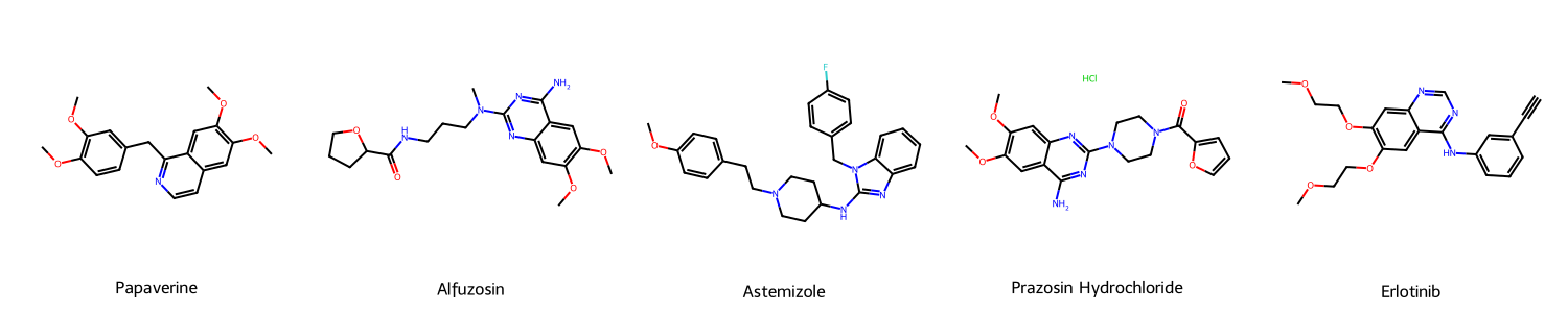
The calculate_similarity_dice function can be used to calculate the Dice similarity metric between two ligands using ECFP/Morgan fingerprints as the similarity measure. The return value is normalized to 1 (1 = 100% similarity, meaning the two compounds are identical) and rounded to two decimal places. The function also provides optional parameters to modify the radius (default: 2) and the bit-vector size (default: 4096) of the generated fingerprints.
Now let’s calculate the similarity between Gefitinib and its analogs we just obtained:
[101]:
for compound in example_analogs:
print(
compound["Name"],
rdkit.calculate_similarity_dice(mol_obj1=example_mol_obj, mol_obj2=compound["MolObj"]),
)
Papaverine 0.34
Alfuzosin 0.35
Astemizole 0.32
Prazosin Hydrochloride 0.35
Erlotinib 0.57
[14:45:37] DEPRECATION WARNING: please use MorganGenerator
[14:45:37] DEPRECATION WARNING: please use MorganGenerator
[14:45:37] DEPRECATION WARNING: please use MorganGenerator
[14:45:37] DEPRECATION WARNING: please use MorganGenerator
[14:45:37] DEPRECATION WARNING: please use MorganGenerator
[14:45:37] DEPRECATION WARNING: please use MorganGenerator
[14:45:37] DEPRECATION WARNING: please use MorganGenerator
[14:45:37] DEPRECATION WARNING: please use MorganGenerator
[14:45:37] DEPRECATION WARNING: please use MorganGenerator
[14:45:37] DEPRECATION WARNING: please use MorganGenerator
Notice that we queried PubChem for compounds with at least 70% similarity to Gefitinib. However, when we calculate the similarities, we see that they are mostly much lower than 70%. The reason is that PubChem uses a different similarity measure and metric than what we do here, i.e. a custom substructure fingerprint with the Tanimoto similarity measure.
Even if we slightly change the settings for generating the Morgan fingerprints, we see that we get different results as well:
[102]:
for compound in example_analogs:
print(
compound["Name"],
rdkit.calculate_similarity_dice(
mol_obj1=example_mol_obj,
mol_obj2=compound["MolObj"],
morgan_radius=3,
morgan_nbits=2048,
),
)
Papaverine 0.28
Alfuzosin 0.28
Astemizole 0.27
Prazosin Hydrochloride 0.29
Erlotinib 0.52
[14:45:37] DEPRECATION WARNING: please use MorganGenerator
[14:45:37] DEPRECATION WARNING: please use MorganGenerator
[14:45:37] DEPRECATION WARNING: please use MorganGenerator
[14:45:37] DEPRECATION WARNING: please use MorganGenerator
[14:45:37] DEPRECATION WARNING: please use MorganGenerator
[14:45:37] DEPRECATION WARNING: please use MorganGenerator
[14:45:37] DEPRECATION WARNING: please use MorganGenerator
[14:45:37] DEPRECATION WARNING: please use MorganGenerator
[14:45:37] DEPRECATION WARNING: please use MorganGenerator
[14:45:37] DEPRECATION WARNING: please use MorganGenerator
Our rdkit module also provide a function calculate_druglikeness, which can be used to obtain several molecular properties, along with four drug-likeness scores:
drug_score_lipinski: based on Lipinski’s rule of 5, normalized to 1 (i.e. 4 = 1, 3 = 0.75, 2 = 0.5, 1 = 0.25, 0 = 0).drug_score_custom: Quantitative Estimate of Drug-likeness (QED) calculated by implementing functions that fit experimental data from G. Bickerton et al., Nat. Chem 2012, 4(2), 90-98..drug_score_qed: QED calculated by ``RDKit` <https://www.rdkit.org/docs/source/rdkit.Chem.QED.html>`__ using default parameters.drug_score_total: weighted average of the above three drug-likeness scores, with a ratio of 1:2:3, respectively.
[103]:
rdkit.calculate_druglikeness(mol_obj=example_mol_obj)
[103]:
{'mol_weight': 446.91,
'num_H_acceptors': 7,
'num_H_donors': 1,
'logp': 4.28,
'tpsa': 68.74,
'num_rot_bonds': 8,
'saturation': 0.36,
'drug_score_qed': 0.52,
'drug_score_lipinski': 1.0,
'drug_score_custom': np.float64(0.56),
'drug_score_total': np.float64(0.61)}
Lastly, we can use the save_3D_molecule_to_SDfile function which prepares a molecule for docking calcluations i.e. adds hydrogen atoms, creates 3D conformation, runs energy minimizations, and saves the result as an SDF file:
[104]:
rdkit.save_3D_molecule_to_SDfile(
mol_obj=example_mol_obj, filepath=example_output_path / "gefitinib"
)
Demonstration of the dogsitescorer helper module
This module implements the API of the DoGSiteScorer functionality of the ProteinsPlus webserver. It can be used to submit protein binding site detection jobs and process the results in order to select a suitable binding site in the target protein. The functions here are used in the BindingSiteDetection class of the pipeline.
[105]:
from utils.helpers import dogsitescorer
To submit a binding site detection job, we can use the function submit_job by providing a valid PDB-code.
[106]:
example_binding_site_data = dogsitescorer.submit_job(
pdb_id="3W32",
ligand_id="W32_A_1101",
chain_id="A",
)
example_binding_site_data
[106]:
| lig_cov | poc_cov | lig_name | volume | enclosure | surface | depth | surf/vol | lid/hull | ellVol | ... | PRO | SER | THR | TRP | TYR | VAL | simpleScore | drugScore | pdb_file_url | ccp4_file_url | |
|---|---|---|---|---|---|---|---|---|---|---|---|---|---|---|---|---|---|---|---|---|---|
| name | |||||||||||||||||||||
| P_0 | 85.48 | 31.22 | W32_A_1101 | 1422.66 | 0.10 | 1673.75 | 19.26 | 1.176493 | - | - | ... | 3 | 1 | 2 | 1 | 1 | 5 | 0.63 | 0.810023 | https://proteins.plus/results/dogsite/fvaKtdhv... | https://proteins.plus/results/dogsite/fvaKtdhv... |
| P_0_0 | 85.48 | 73.90 | W32_A_1101 | 599.23 | 0.06 | 540.06 | 17.51 | 0.901257 | - | - | ... | 1 | 0 | 2 | 0 | 0 | 2 | 0.59 | 0.620201 | https://proteins.plus/results/dogsite/fvaKtdhv... | https://proteins.plus/results/dogsite/fvaKtdhv... |
| P_0_1 | 3.23 | 0.44 | W32_A_1101 | 201.73 | 0.08 | 381.07 | 11.36 | 1.889010 | - | - | ... | 0 | 0 | 1 | 0 | 0 | 1 | 0.17 | 0.174816 | https://proteins.plus/results/dogsite/fvaKtdhv... | https://proteins.plus/results/dogsite/fvaKtdhv... |
| P_0_2 | 0.00 | 0.00 | W32_A_1101 | 185.60 | 0.17 | 282.00 | 9.35 | 1.519397 | - | - | ... | 0 | 0 | 0 | 0 | 0 | 2 | 0.13 | 0.195695 | https://proteins.plus/results/dogsite/fvaKtdhv... | https://proteins.plus/results/dogsite/fvaKtdhv... |
| P_0_3 | 6.45 | 0.29 | W32_A_1101 | 175.30 | 0.15 | 297.42 | 9.29 | 1.696634 | - | - | ... | 1 | 1 | 0 | 0 | 0 | 1 | 0.13 | 0.168845 | https://proteins.plus/results/dogsite/fvaKtdhv... | https://proteins.plus/results/dogsite/fvaKtdhv... |
| P_0_4 | 0.00 | 0.00 | W32_A_1101 | 170.37 | 0.08 | 390.10 | 11.99 | 2.289722 | - | - | ... | 0 | 0 | 0 | 1 | 1 | 0 | 0.15 | 0.223742 | https://proteins.plus/results/dogsite/fvaKtdhv... | https://proteins.plus/results/dogsite/fvaKtdhv... |
| P_0_5 | 0.00 | 0.00 | W32_A_1101 | 90.43 | 0.24 | 177.50 | 6.24 | 1.962844 | - | - | ... | 1 | 0 | 0 | 0 | 0 | 2 | 0.00 | 0.165232 | https://proteins.plus/results/dogsite/fvaKtdhv... | https://proteins.plus/results/dogsite/fvaKtdhv... |
| P_1 | 0.00 | 0.00 | W32_A_1101 | 708.99 | 0.13 | 1030.19 | 14.32 | 1.453039 | - | - | ... | 1 | 2 | 2 | 0 | 1 | 1 | 0.46 | 0.755915 | https://proteins.plus/results/dogsite/fvaKtdhv... | https://proteins.plus/results/dogsite/fvaKtdhv... |
| P_1_0 | 0.00 | 0.00 | W32_A_1101 | 496.90 | 0.11 | 739.17 | 12.72 | 1.487563 | - | - | ... | 1 | 2 | 2 | 0 | 1 | 1 | 0.49 | 0.465489 | https://proteins.plus/results/dogsite/fvaKtdhv... | https://proteins.plus/results/dogsite/fvaKtdhv... |
| P_1_1 | 0.00 | 0.00 | W32_A_1101 | 212.10 | 0.16 | 454.31 | 11.03 | 2.141961 | - | - | ... | 0 | 0 | 0 | 0 | 1 | 0 | 0.19 | 0.242990 | https://proteins.plus/results/dogsite/fvaKtdhv... | https://proteins.plus/results/dogsite/fvaKtdhv... |
| P_2 | 0.00 | 0.00 | W32_A_1101 | 286.21 | 0.18 | 462.29 | 11.83 | 1.615213 | - | - | ... | 2 | 0 | 1 | 0 | 1 | 3 | 0.09 | 0.537137 | https://proteins.plus/results/dogsite/fvaKtdhv... | https://proteins.plus/results/dogsite/fvaKtdhv... |
| P_2_0 | 0.00 | 0.00 | W32_A_1101 | 148.16 | 0.15 | 271.11 | 10.75 | 1.829846 | - | - | ... | 2 | 0 | 0 | 0 | 1 | 2 | 0.06 | 0.278636 | https://proteins.plus/results/dogsite/fvaKtdhv... | https://proteins.plus/results/dogsite/fvaKtdhv... |
| P_2_1 | 0.00 | 0.00 | W32_A_1101 | 138.05 | 0.20 | 320.52 | 7.29 | 2.321767 | - | - | ... | 1 | 0 | 1 | 0 | 0 | 1 | 0.05 | 0.244429 | https://proteins.plus/results/dogsite/fvaKtdhv... | https://proteins.plus/results/dogsite/fvaKtdhv... |
| P_3 | 0.00 | 0.00 | W32_A_1101 | 244.16 | 0.04 | 514.94 | 14.34 | 2.109027 | - | - | ... | 3 | 2 | 1 | 0 | 1 | 1 | 0.12 | 0.572013 | https://proteins.plus/results/dogsite/fvaKtdhv... | https://proteins.plus/results/dogsite/fvaKtdhv... |
| P_4 | 0.00 | 0.00 | W32_A_1101 | 169.28 | 0.21 | 373.47 | 11.49 | 2.206226 | - | - | ... | 2 | 0 | 1 | 0 | 0 | 0 | 0.07 | 0.424397 | https://proteins.plus/results/dogsite/fvaKtdhv... | https://proteins.plus/results/dogsite/fvaKtdhv... |
| P_4_0 | 0.00 | 0.00 | W32_A_1101 | 108.35 | 0.22 | 237.70 | 7.50 | 2.193816 | - | - | ... | 0 | 0 | 0 | 0 | 0 | 0 | 0.02 | 0.355261 | https://proteins.plus/results/dogsite/fvaKtdhv... | https://proteins.plus/results/dogsite/fvaKtdhv... |
| P_4_1 | 0.00 | 0.00 | W32_A_1101 | 60.93 | 0.20 | 193.96 | 5.80 | 3.183325 | - | - | ... | 2 | 0 | 1 | 0 | 0 | 0 | 0.00 | 0.570708 | https://proteins.plus/results/dogsite/fvaKtdhv... | https://proteins.plus/results/dogsite/fvaKtdhv... |
| P_5 | 0.00 | 0.00 | W32_A_1101 | 166.59 | 0.16 | 347.46 | 11.99 | 2.085719 | - | - | ... | 1 | 1 | 0 | 0 | 1 | 0 | 0.00 | 0.401384 | https://proteins.plus/results/dogsite/fvaKtdhv... | https://proteins.plus/results/dogsite/fvaKtdhv... |
| P_6 | 0.00 | 0.00 | W32_A_1101 | 155.14 | 0.00 | 146.79 | 11.39 | 0.946178 | - | - | ... | 1 | 3 | 1 | 2 | 1 | 2 | 0.00 | 0.399009 | https://proteins.plus/results/dogsite/fvaKtdhv... | https://proteins.plus/results/dogsite/fvaKtdhv... |
| P_7 | 0.00 | 0.00 | W32_A_1101 | 116.03 | 0.27 | 227.72 | 8.04 | 1.962596 | - | - | ... | 1 | 0 | 0 | 1 | 1 | 0 | 0.00 | 0.224937 | https://proteins.plus/results/dogsite/fvaKtdhv... | https://proteins.plus/results/dogsite/fvaKtdhv... |
| P_8 | 0.00 | 0.00 | W32_A_1101 | 105.98 | 0.23 | 206.04 | 10.16 | 1.944140 | - | - | ... | 2 | 0 | 0 | 1 | 1 | 0 | 0.00 | 0.308046 | https://proteins.plus/results/dogsite/fvaKtdhv... | https://proteins.plus/results/dogsite/fvaKtdhv... |
| P_9 | 0.00 | 0.00 | W32_A_1101 | 104.32 | 0.09 | 202.13 | 9.20 | 1.937596 | - | - | ... | 0 | 1 | 0 | 0 | 1 | 1 | 0.00 | 0.267262 | https://proteins.plus/results/dogsite/fvaKtdhv... | https://proteins.plus/results/dogsite/fvaKtdhv... |
22 rows × 51 columns
Notice that the submit_job function can also take in a chain-ID to limit the detection on that specific chain, and a ligand-ID to also calculate the coverage of each detected binding site. However, the ligand-ID that DoGSiteScorer accepts has its own format and is not the same as the ligand-ID in the protein PDB file.
Nevertheless, it follows the following format: (ligand-ID)_(chain-ID)_(ligand-residue-ID). When implementing the BindingSiteDetection class, we will circumvent this by automatically generating the DogSiteScorer ligand-ID from the normal ligand-ID so that the user does not have to manually look up and enter the ligand-ID in this specific format.
If we want to detect the binding sites of a protein from a local PDB file, we should first upload the file to the DogSiteScorer webserver using the upload_pdb_file function; it returns a dummy PDB-code for the uploaded structure, which can be used in place of a valid PDB-code to submit a binding site detection job. For this, we will use the PDB file we downloaded earlier.
Note: This process should take about one minute to complete. We recently experienced very long processing times, so the following line may raise ValueError: Fetching results from DoGSiteScorer API failed.
[107]:
# NBVAL_SKIP
example_dummy_pdb_id = dogsitescorer.upload_pdb_file(filepath=example_downloaded_protein_filepath)
example_dummy_pdb_id
[107]:
'3w32pdbf1458ec7-364d-4616-b560-8f4211db271e'
[108]:
# NBVAL_SKIP
dogsitescorer.submit_job(pdb_id=example_dummy_pdb_id, ligand_id="W32_A_1101", chain_id="A").head()
[108]:
| lig_cov | poc_cov | lig_name | volume | enclosure | surface | depth | surf/vol | lid/hull | ellVol | ... | PRO | SER | THR | TRP | TYR | VAL | simpleScore | drugScore | pdb_file_url | ccp4_file_url | |
|---|---|---|---|---|---|---|---|---|---|---|---|---|---|---|---|---|---|---|---|---|---|
| name | |||||||||||||||||||||
| P_0 | 85.48 | 31.22 | W32_A_1101 | 1422.66 | 0.10 | 1673.75 | 19.26 | 1.176493 | - | - | ... | 3 | 1 | 2 | 1 | 1 | 5 | 0.63 | 0.810023 | https://proteins.plus/results/dogsite/WB8aXgzh... | https://proteins.plus/results/dogsite/WB8aXgzh... |
| P_0_0 | 85.48 | 73.90 | W32_A_1101 | 599.23 | 0.06 | 540.06 | 17.51 | 0.901257 | - | - | ... | 1 | 0 | 2 | 0 | 0 | 2 | 0.59 | 0.620201 | https://proteins.plus/results/dogsite/WB8aXgzh... | https://proteins.plus/results/dogsite/WB8aXgzh... |
| P_0_1 | 3.23 | 0.44 | W32_A_1101 | 201.73 | 0.08 | 381.07 | 11.36 | 1.889010 | - | - | ... | 0 | 0 | 1 | 0 | 0 | 1 | 0.17 | 0.174816 | https://proteins.plus/results/dogsite/WB8aXgzh... | https://proteins.plus/results/dogsite/WB8aXgzh... |
| P_0_2 | 0.00 | 0.00 | W32_A_1101 | 185.60 | 0.17 | 282.00 | 9.35 | 1.519397 | - | - | ... | 0 | 0 | 0 | 0 | 0 | 2 | 0.13 | 0.195695 | https://proteins.plus/results/dogsite/WB8aXgzh... | https://proteins.plus/results/dogsite/WB8aXgzh... |
| P_0_3 | 6.45 | 0.29 | W32_A_1101 | 175.30 | 0.15 | 297.42 | 9.29 | 1.696634 | - | - | ... | 1 | 1 | 0 | 0 | 0 | 1 | 0.13 | 0.168845 | https://proteins.plus/results/dogsite/WB8aXgzh... | https://proteins.plus/results/dogsite/WB8aXgzh... |
5 rows × 51 columns
The submit_job function returns a DataFrame containing all the detected binding pockets and their respective properties. It also contains the URLs of the PDB and CCP4 files for each of the detected binding pockets, which can be used to download the files later.
Among the calculated properties, the most important are (for more details, see A. Volkamer et al., J. Chem. Inf. Model. 2012, 52, 360-372.):
druggability scores (between 0 and 1; the higher the score the more druggable the binding site):
simpleScore: simple druggability score, based on a linear combination of the three descriptors describing volume, hydrophobicity and enclosure.drugScore: druggability score derived by incorporation of a subset of meaningful descriptors in a support vector machine (libsvm).ligand coverage data (for when a ligand-ID is also specified in the job submission)
lig_cov: the percentage of the ligand volume that is covered by the pocket.poc_cov: percentage of the binding site volume that is covered by the ligand.volume: volume of the pocket in Å3.
The list of all properties can be accessed by retrieving the column names of the DataFrame:
[109]:
example_binding_site_data.columns
[109]:
Index(['lig_cov', 'poc_cov', 'lig_name', 'volume', 'enclosure', 'surface',
'depth', 'surf/vol', 'lid/hull', 'ellVol', 'ell c/a', 'ell b/a',
'siteAtms', 'accept', 'donor', 'hydrophobic_interactions',
'hydrophobicity', 'metal', 'Cs', 'Ns', 'Os', 'Ss', 'Xs', 'negAA',
'posAA', 'polarAA', 'apolarAA', 'ALA', 'ARG', 'ASN', 'ASP', 'CYS',
'GLN', 'GLU', 'GLY', 'HIS', 'ILE', 'LEU', 'LYS', 'MET', 'PHE', 'PRO',
'SER', 'THR', 'TRP', 'TYR', 'VAL', 'simpleScore', 'drugScore',
'pdb_file_url', 'ccp4_file_url'],
dtype='object')
Depending on the specifics of the project, these values can be used to select the most-suitable detected binding site. Here, we have implemented two possibilities for this selection process in the select_best_pocket function.
The first option is to provide a list of properties in order of importance, based on which the binding site with the highest or lowest value is to be chosen. The function then returns the name of the selected binding site.
The list of properties should be inputted as a list. For example, the selection_criteria argument below sorts the binding sites by their lig_cov values and if there are two or more binding sites with the same lig_cov value, it then sorts them by their poc_cov values:
[110]:
example_best_pocket_name = dogsitescorer.select_best_pocket(
binding_site_df=example_binding_site_data,
selection_method="sorting",
selection_criteria=["lig_cov", "poc_cov"],
ascending=False,
)
example_best_pocket_name
[110]:
'P_0_0'
Another possibility for selecting a binding site is to provide any valid Python expression that generates a list-like object with the same length as the number of detected binding sites. This Python expression is taken in as a string and evaluated during the runtime, so the user can directly input a Python expression in the input CSV file.
For example, using this method we can perform any calculation on the properties in the binding site dataframe.
Note: for referring to the binding site dataframe, df should be used:
[111]:
dogsitescorer.select_best_pocket(
binding_site_df=example_binding_site_data,
selection_method="function",
selection_criteria="((df['lig_cov'] + df['poc_cov']) / 2) * ((df['drugScore'] + df['simpleScore']) / 2) / df['volume']",
ascending=False,
)
[111]:
'P_0_0'
For example, the above selection_criteria is a function that calculates the average of lig_cov and poc_cov, as well as the average of drugScore and simpleScore, multiplies the two together and then divides the result by the volume. The binding site that has the highest value is then chosen. If we want to have the lowest value, we can set the ascending parameter to False.
Another example is:
[112]:
dogsitescorer.select_best_pocket(
binding_site_df=example_binding_site_data,
selection_method="function",
selection_criteria="df[['drugScore', 'simpleScore']].min(axis=1) * df[['poc_cov', 'lig_cov']].max(axis=1)",
ascending=False,
)
[112]:
'P_0'
The above example calculates the minimum value between drugScore and simpleScore, and multiplies the results with the maximum value between the poc_cov and lig_cov.
We now want to calculate the coordinates of the selected binding site to use in the docking process. For this, we first need to download the PDB files of the detected binding sites, using the save_binding_sites_to_file function. It files will be saved in the given output_path under the same name as their corresponding pocket:
[113]:
dogsitescorer.save_binding_sites_to_file(
binding_site_df=example_binding_site_data, output_path=example_output_path
)
Having downloaded the necessary binding site files, we can now calculate the coordinates of the selected pocket by providing the filepath of its data (i.e output_path of the above function + selected pocket’s name) to the calculate_pocket_coordinates_from_pocket_pdb_file function:
[114]:
dogsitescorer.calculate_pocket_coordinates_from_pocket_pdb_file(
filepath=example_output_path / example_best_pocket_name
)
[114]:
{'center': [15.91, 32.33, 11.03], 'size': [24.84, 24.84, 24.84]}
Lastly, we can also see which residues comprise a certain pocket by providing the pocket’s downloaded PDB filepath to the function get_pocket_residues:
[115]:
dogsitescorer.get_pocket_residues(
pocket_pdb_filepath=example_output_path / example_best_pocket_name
)
[115]:
| residue_number | residue_name | |
|---|---|---|
| 1 | 718 | LEU |
| 2 | 726 | VAL |
| 3 | 743 | ALA |
| 4 | 744 | ILE |
| 5 | 745 | LYS |
| 6 | 766 | MET |
| 7 | 769 | VAL |
| 8 | 775 | CYS |
| 9 | 776 | ARG |
| 10 | 777 | LEU |
| 11 | 788 | LEU |
| 12 | 789 | ILE |
| 13 | 790 | THR |
| 14 | 791 | GLN |
| 15 | 792 | LEU |
| 16 | 793 | MET |
| 17 | 794 | PRO |
| 18 | 796 | GLY |
| 19 | 797 | CYS |
| 20 | 841 | ARG |
| 21 | 842 | ASN |
| 22 | 844 | LEU |
| 23 | 854 | THR |
| 24 | 855 | ASP |
| 25 | 856 | PHE |
| 26 | 857 | GLY |
| 27 | 858 | LEU |
| 28 | 997 | PHE |
| 29 | 1001 | LEU |
Demonstration of the obabel helper module
Here you will find functions needed to prepare the protein and the ligand analogs for docking, e.g. by adding missing hydrogen atoms, defining protonation states based on a given pH value, determining partial charges, generating a low-energy conformation of ligands, and saving its coordinates as a PDBQT file. These are implemented with the help of pybel module of the openbabel package.
This helper module also provides functions for splitting multi-structure files, or merging several files into a multi-structure file. These are useful, e.g. for processing the docking output files later, and are used in the Docking and InteractionAnalysis classes of the pipeline.
[116]:
from utils.helpers import obabel
The function optimize_structure_for_docking can be used to prepare a structure for docking. It takes in an openbabel.pybel.Molecule object, and modifies it in place to — depending on the specified parameters — add hydrogen atoms to the structure, correct the protonation state of each atom based on a given pH value, calculate partial charges, and generate a force-field-optimized 3D conformation.
However, unless you wish to work with your own openbabel.pybel.Molecule object, there is no need to use this function directly, as it is also implemented in the functions create_pdbqt_from_smiles and create_pdbqt_from_pdb_file.
Let’s create a PDBQT file for Gefitinib from its SMILES:
[117]:
obabel.create_pdbqt_from_smiles(
smiles="COC1=C(C=C2C(=C1)N=CN=C2NC3=CC(=C(C=C3)F)Cl)OCCCN4CCOCC4",
pdbqt_path=example_output_path / "gefitinib",
)
And one for our extracted protein:
[118]:
obabel.create_pdbqt_from_pdb_file(
pdb_filepath=example_output_path / "extracted_protein.pdb",
pdbqt_filepath=example_output_path / "extracted_protein.pdbqt",
)
Other functions in this module include split_multistructure_file, which allows you to split a multi-structure file (e.g. PDB, PDBQT, SDF) into several files of the same type, each containing a single structure. We will use this function in the section demonstrating the plip helper module, to separate the docking poses of a ligand. Also, merge_molecules_to_single_file allows you to do the opposite.
Demonstration of the smina helper module
This module is responsible for communicating with the Smina program via shell commands, in order to perform docking calculations. It also contains a function to process the output log of the program and extract information. The module is used in the Docking class of the pipeline.
[119]:
from utils.helpers import smina
In order to dock a ligand onto a specified pocket of a protein, we can use the function dock. For this, we have to provide the following parameters:
ligand_path: filepath of the ligand PDBQT file.protein_path: filepath of the protein PDBQT file.pocket_center: xyz-coordinates of the pocket’s center (as an iterable of three numbers).pocket_size: xyz-lenghts of the pocket (as an iterable of three numbers).output_path: filepath to save the docking poses in.
There are also several optional parameters that we can modify:
output_format: file format corresponding tooutput_path(default: PDBQT).num_poses: maximum number of docking poses to generate (default: 10).exhaustiveness: exhaustiveness of the global search (roughy proportional to time), which influences the accuracy of the docking calculations (default: 10).random_seed: explicit seed phrase to make the docking results deterministic for reproducibility (default: None)log: whether to also write a log file in the same path asoutput_path(default: True)
[120]:
example_smina_output = smina.dock(
ligand_path=example_output_path / "gefitinib.pdbqt",
protein_path=example_output_path / "extracted_protein.pdbqt",
pocket_center=[15.91, 32.33, 11.03],
pocket_size=[24.84, 24.84, 24.84],
output_path=example_output_path / "docking",
output_format="pdbqt",
num_poses=5,
exhaustiveness=10,
random_seed=1111,
log=True,
)
example_smina_output
[120]:
' _______ _______ _________ _ _______ \n ( ____ \\( )\\__ __/( ( /|( ___ )\n | ( \\/| () () | ) ( | \\ ( || ( ) |\n | (_____ | || || | | | | \\ | || (___) |\n (_____ )| |(_)| | | | | (\\ \\) || ___ |\n ) || | | | | | | | \\ || ( ) |\n /\\____) || ) ( |___) (___| ) \\ || ) ( |\n \\_______)|/ \\|\\_______/|/ )_)|/ \\|\n\n\nsmina is based off AutoDock Vina. Please cite appropriately.\n\nWeights Terms\n-0.035579 gauss(o=0,_w=0.5,_c=8)\n-0.005156 gauss(o=3,_w=2,_c=8)\n0.840245 repulsion(o=0,_c=8)\n-0.035069 hydrophobic(g=0.5,_b=1.5,_c=8)\n-0.587439 non_dir_h_bond(g=-0.7,_b=0,_c=8)\n1.923 num_tors_div\n\nUsing random seed: 1111\n\n0% 10 20 30 40 50 60 70 80 90 100%\n|----|----|----|----|----|----|----|----|----|----|\n***************************************************\n\nmode | affinity | dist from best mode\n | (kcal/mol) | rmsd l.b.| rmsd u.b.\n-----+------------+----------+----------\n1 -8.9 0.000 0.000 \n2 -8.8 2.144 5.515 \n3 -8.7 1.892 4.945 \n4 -8.6 4.715 8.268 \n5 -8.5 2.661 6.196 \nRefine time 29.295\nLoop time 34.171\n'
Now to better analyze and process the docking results, we can use the function convert_log_to_dataframe to generate a dataframe from Smina’s output log:
[121]:
example_docking_df = smina.convert_log_to_dataframe(example_smina_output)
example_docking_df
[121]:
| affinity[kcal/mol] | dist from best mode_rmsd_l.b | dist from best mode_rmsd_u.b | |
|---|---|---|---|
| mode | |||
| 1 | -8.9 | 0.000 | 0.000 |
| 2 | -8.8 | 2.144 | 5.515 |
| 3 | -8.7 | 1.892 | 4.945 |
| 4 | -8.6 | 4.715 | 8.268 |
| 5 | -8.5 | 2.661 | 6.196 |
Demonstration of the plip helper module
Implemented in this module are the functions necessary for calculating protein—ligand interactions using the plip package, and analyzing the results. It is used in the class InteractionAnalysis of the pipeline.
[122]:
from utils.helpers import plip
In order to analyze the interactions in the generated docking poses by smina, we first need to create PDB files containing the protein and a single docking pose.
Since Smina generates a single multi-structure file containing all the docking poses, we first need to split this file. For this, we can use the split_multistructure_file of the obabel module we mentioned before. It splits the structures in the file into single-structure files of the same format, and returns the filepaths:
[123]:
example_docking_poses_filepaths = obabel.split_multistructure_file(
filetype="pdbqt", filepath=example_output_path / "docking.pdbqt"
)
example_docking_poses_filepaths
[123]:
[PosixPath('/Users/sakhawathsumit/Documents/teachopencadd/teachopencadd/talktorials/T018_automated_cadd_pipeline/data/Outputs/Examples/docking_1.pdbqt'),
PosixPath('/Users/sakhawathsumit/Documents/teachopencadd/teachopencadd/talktorials/T018_automated_cadd_pipeline/data/Outputs/Examples/docking_2.pdbqt'),
PosixPath('/Users/sakhawathsumit/Documents/teachopencadd/teachopencadd/talktorials/T018_automated_cadd_pipeline/data/Outputs/Examples/docking_3.pdbqt'),
PosixPath('/Users/sakhawathsumit/Documents/teachopencadd/teachopencadd/talktorials/T018_automated_cadd_pipeline/data/Outputs/Examples/docking_4.pdbqt'),
PosixPath('/Users/sakhawathsumit/Documents/teachopencadd/teachopencadd/talktorials/T018_automated_cadd_pipeline/data/Outputs/Examples/docking_5.pdbqt')]
Now for each docking pose we want to analyze, we need to create a protein-ligand complex as a PDB file. The function create_protein_ligand_complex does just that. Again, it returns the filepath of the created PDB file.
Let’s use the first docking pose (i.e. example_docking_poses_filepaths[0]) to generate a complex:
[124]:
example_complex_filepath = plip.create_protein_ligand_complex(
protein_pdbqt_filepath=example_output_path / "extracted_protein.pdbqt",
docking_pose_pdbqt_filepath=example_docking_poses_filepaths[0],
ligand_id="Gefitinib",
output_filepath=example_output_path / "protein_ligand_complex",
)
example_complex_filepath
[124]:
PosixPath('/Users/sakhawathsumit/Documents/teachopencadd/teachopencadd/talktorials/T018_automated_cadd_pipeline/data/Outputs/Examples/protein_ligand_complex.pdb')
Now we can use the function calculate_interactions to analyze the protein-ligand interactions in this complex. The function returns a dict, where each key corresponds to a ligand, and its value is another dict containing the interaction data:
[125]:
example_interactions = plip.calculate_interactions(pdb_filepath=example_complex_filepath)
example_interactions.keys()
[125]:
dict_keys(['UNL:A:1'])
Since we only had one ligand in our complex, we are only interested in the inside dict:
[126]:
example_interactions = example_interactions[list(example_interactions.keys())[0]]
This dict’s keys each correspond to a specific interaction type:
[127]:
example_interactions.keys()
[127]:
dict_keys(['hbond', 'hydrophobic', 'saltbridge', 'waterbridge', 'pistacking', 'pication', 'halogen', 'metal'])
These interactions types are implemented in the subclass plip.Consts.InteractionTypes as Enum:
[128]:
list(plip.Consts.InteractionTypes)
[128]:
[<InteractionTypes.H_BOND: 'hbond'>,
<InteractionTypes.HYDROPHOBIC: 'hydrophobic'>,
<InteractionTypes.SALT_BRIDGE: 'saltbridge'>,
<InteractionTypes.WATER_BRIDGE: 'waterbridge'>,
<InteractionTypes.PI_STACKING: 'pistacking'>,
<InteractionTypes.PI_CATION: 'pication'>,
<InteractionTypes.HALOGEN: 'halogen'>,
<InteractionTypes.METAL: 'metal'>]
when using Pybel to create the protein PDBQT file for the docking experiment, the residue numbers are reset (i.e. start at 1). Since this PDBQT file is also used to create a PDB file for the protein—ligand complex that PLIP analyzes, the residue numbers in our interaction data are also affected.
To fix this before further processing the data, we use the function correct_protein_residue_numbers and provide the first residue number of our protein. This fixes all residue numbers in the interaction data in-place:
[129]:
example_interactions = plip.correct_protein_residue_numbers(
ligand_interaction_data=example_interactions, protein_first_residue_number=701
)
Now we can use the function create_dataframe_of_ligand_interactions to create a dataframe for each specific interaction type, by providing its Enum.
For example, to create a dataframe for hydrophobic interactions present in example_interactions:
[130]:
plip.create_dataframe_of_ligand_interactions(
ligand_interaction_data=example_interactions,
interaction_type=plip.Consts.InteractionTypes.HYDROPHOBIC,
)
[130]:
| RESNR | RESTYPE | RESCHAIN | RESNR_LIG | RESTYPE_LIG | RESCHAIN_LIG | DIST | LIGCARBONIDX | PROTCARBONIDX | LIGCOO | PROTCOO | |
|---|---|---|---|---|---|---|---|---|---|---|---|
| 0 | 726 | VAL | A | 1 | UNL | A | 3.54 | 3098 | 2474 | (16.9, 34.028, 10.662) | (19.4, 36.488, 11.163) |
| 1 | 841 | ARG | A | 1 | UNL | A | 3.76 | 3088 | 2995 | (21.621, 32.884, 16.004) | (22.764, 29.723, 17.692) |
| 2 | 854 | THR | A | 1 | UNL | A | 3.84 | 3102 | 3065 | (17.953, 31.867, 10.524) | (16.714, 28.916, 12.649) |
| 3 | 855 | ASP | A | 1 | UNL | A | 3.89 | 3102 | 3068 | (17.953, 31.867, 10.524) | (19.977, 28.578, 10.059) |
Demonstration of the nglview helper module
This module uses the NGLview Jupyter widget to implement functions for visualization of protein related data, such as the protein structure itself, protein binding sites, docking poses inside the protein and their interactions with specific residues. It is used in several classes of the pipeline, e.g. Protein, Docking and InteractionAnalysis.
[131]:
from utils.helpers import nglview
We can visualize a protein structure using its PDB-code or local PDB filepath, by using the function protein. If we provide an output_image_filename, a static image of the protein will also be downloaded:
[132]:
nglview.protein(input_type="pdb_code", input_value="3w32")
Sending GET request to https://files.rcsb.org/download/3w32.pdb to fetch 3w32's pdb file as a string.
The function binding_site can visualize a binding pocket in the protein. We must provide the protein structure (either as PDB-code or PDB file) and the CCP4 file describing the binding pocket (generated by DoGSiteScorer):
[133]:
nglview.binding_site(
protein_input_type="pdb_code",
protein_input_value="3W32",
ccp4_filepath=example_output_path / example_best_pocket_name,
)
Sending GET request to https://files.rcsb.org/download/3W32.pdb to fetch 3W32's pdb file as a string.
To view docking poses, we can use the function docking, which requires the following parameters:
protein_filepath: filepath of the extracted protein structure used in docking.list_docking_poses_filepaths: list of filepaths for all docking poses to be viewed. Each file must contain a single docking pose.list_docking_poses_labels: list of labels for the provided docking poses to distinguish them in the generated menu.list_docking_poses_affinities: list of calculated binding affinities for the provided docking poses to add to the view.
[134]:
view = nglview.docking(
protein_filepath=example_output_path / "extracted_protein.pdb",
list_docking_poses_filepaths=example_docking_poses_filepaths,
list_docking_poses_labels=list(
map((lambda index: "123631 - " + str(index)), example_docking_df.index.values)
),
list_docking_poses_affinities=example_docking_df["affinity[kcal/mol]"].values,
)
Docking modes
(CID - mode)
Similarly, we can use the function interactions to visualize the protein-ligand interactions in each docking pose. Here we should also provide the same parameters as in nglview.docking, with the addition of list_docking_poses_plip_dicts, which should be a list containing the interaction data for each docking pose created by plip:
[135]:
nglview.interactions(
protein_filepath=example_output_path / "extracted_protein.pdb",
list_docking_poses_filepaths=example_docking_poses_filepaths[0:1],
list_docking_poses_labels=list(
map((lambda index: "123631 - " + str(index)), example_docking_df.index.values)
),
list_docking_poses_affinities=example_docking_df["affinity[kcal/mol]"].values,
list_docking_poses_plip_dicts=[example_interactions],
)

[135]: