T027 · Kinase similarity: Ligand profile
Note: This talktorial is a part of TeachOpenCADD, a platform that aims to teach domain-specific skills and to provide pipeline templates as starting points for research projects.
Authors:
Talia B. Kimber, 2021, Volkamer lab, Charité
Dominique Sydow, 2021, Volkamer lab, Charité
Andrea Volkamer, 2021, Volkamer lab, Charité
Aim of this talktorial
The aim of this talktorial is to investigate kinase similarity through ligand profiling data (ChEMBL29). In the context of drug design, the following assumption is often made: if a compound was tested active on two different kinases, it is suspected that these two kinases may have some degree of similarity. We will use this assumption in this talktorial. The concept of kinase promiscuity is also covered.
Contents in Theory
Kinase dataset
Bioactivity data
Kinase similarity descriptor: Ligand profile
Kinase similarity
Kinase promiscuity
From similarity matrix to distance matrix
Contents in Practical
Define the kinases of interest
Retrieve the data
Preprocess the data
Hit or non-hit
Kinase promiscuity
Kinase similarity
Visualize similarity as kinase matrix
Save kinase similarity matrix
Kinase distance matrix
Save kinase distance matrix
References
Kinase dataset: Molecules (2021), 26(3), 629
ChEMBL database
KinMap
Website: http://www.kinhub.org/kinmap/
[1]:
import sys

if "google.colab" in sys.modules:
    %pip install teachopencadd --no-deps -q
    !teachopencadd -d 27
    %pip uninstall teachopencadd -y -q
    %pip install -qr requirements.txt
Theory
Kinase dataset
We use the kinase selection as defined in Talktorial T023.
Bioactivity data
In order to measure kinase similarity through ligand profiling data, bioactivity data is retrieved from the well-known ChEMBL database and the query focuses on human kinases. Luckily, a curated version of ChEMBL29 is already freely available through the Openkinome organization, see https://github.com/openkinome/kinodata. For more details on querying the ChEMBL database, please refer to Talktorial T001.
In drug design, it is common to binarize the activity of a compound against a target of interest as a “hit” or “non-hit”. Practically speaking, this is done using a cutoff value for measured activity. If the activity is greater than the cutoff, the compound is labeled as active (hit), and inactive (non-hit) otherwise.
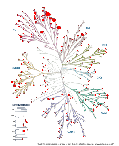
Figure 1: Number of ChEMBL29 bioactivities per kinase - as collected in kinodata - mapped onto the Manning kinome tree using KinMap. The figure has been generated in Talktorial T023.
Kinase similarity descriptor: Ligand profile
As a measure of similarity, we use ligand profiling data in this talktorial.
Kinase similarity
We use the following metric as similarity between two kinases \(K_i\) and \(K_j\) :
Assuming that only one compound was tested on two kinases, and that the compound was tested as active for one and inactive for the other, then the similarity between these two kinases would be zero.
Kinase promiscuity
Computing the similarity between a kinase and itself may be interpreted as kinase promiscuity, where the similarity described above would therefore represent the fraction of active compounds over all tested compounds.
From similarity matrix to distance matrix
As discussed in Talktorial T024, we convert the similarity matrix to a distance matrix.
Practical
[2]:
from pathlib import Path
from collections import Counter

import pandas as pd
import numpy as np
import seaborn as sns
import matplotlib.pyplot as plt

from rdkit import Chem
from rdkit.Chem import Draw
from rdkit.Chem.Draw import IPythonConsole
[3]:
HERE = Path(_dh[-1])
DATA = HERE / "data"
[4]:
configs = pd.read_csv(DATA / "pipeline_configs.csv")
configs = configs.set_index("variable")["default_value"]
DEMO = bool(int(configs["DEMO"]))
print(f"Run in demo mode: {DEMO}")
# NBVAL_CHECK_OUTPUT
Run in demo mode: True
Define the kinases of interest
Let’s load the kinase selection as defined in Talktorial T023.
[5]:
kinase_selection_df = pd.read_csv(DATA / "kinase_selection.csv")
kinase_selection_df
# NBVAL_CHECK_OUTPUT
[5]:
| kinase | kinase_klifs | uniprot_id | group | full_kinase_name | |
|---|---|---|---|---|---|
| 0 | EGFR | EGFR | P00533 | TK | Epidermal growth factor receptor |
| 1 | ErbB2 | ErbB2 | P04626 | TK | Erythroblastic leukemia viral oncogene homolog 2 |
| 2 | PI3K | p110a | P42336 | Atypical | Phosphatidylinositol-3-kinase |
| 3 | VEGFR2 | KDR | P35968 | TK | Vascular endothelial growth factor receptor 2 |
| 4 | BRAF | BRAF | P15056 | TKL | Rapidly accelerated fibrosarcoma isoform B |
| 5 | CDK2 | CDK2 | P24941 | CMGC | Cyclic-dependent kinase 2 |
| 6 | LCK | LCK | P06239 | TK | Lymphocyte-specific protein tyrosine kinase |
| 7 | MET | MET | P08581 | TK | Mesenchymal-epithelial transition factor |
| 8 | p38a | p38a | Q16539 | CMGC | p38 mitogen activated protein kinase alpha |
Retrieve the data
We retrieve a pre-curated version of a kinase subset of ChEMBL29 freely available at Openkinome, see https://github.com/openkinome/kinodata/releases/tag/v0.3.
[6]:
path = "https://github.com/openkinome/kinodata/releases/download/\
v0.3/activities-chembl29_v0.3.zip"
# Load data and reset index so that it starts from 0
data = pd.read_csv(path, index_col=0).reset_index(drop=True)
print(f"Current shape of data: {data.shape}")
data.head()
# NBVAL_CHECK_OUTPUT
Current shape of data: (190634, 16)
[6]:
| activities.activity_id | assays.chembl_id | target_dictionary.chembl_id | molecule_dictionary.chembl_id | molecule_dictionary.max_phase | activities.standard_type | activities.standard_value | activities.standard_units | compound_structures.canonical_smiles | compound_structures.standard_inchi | component_sequences.sequence | assays.confidence_score | docs.chembl_id | docs.year | docs.authors | UniprotID | |
|---|---|---|---|---|---|---|---|---|---|---|---|---|---|---|---|---|
| 0 | 16291323 | CHEMBL3705523 | CHEMBL2973 | CHEMBL3666724 | 0 | pIC50 | 14.096910 | nM | CCCC(=O)Nc1cccc(-c2nc(Nc3ccc4[nH]ncc4c3)c3cc(O... | InChI=1S/C31H33N7O3/c1-2-4-29(40)33-22-6-3-5-2... | MSRPPPTGKMPGAPETAPGDGAGASRQRKLEALIRDPRSPINVESL... | 9 | CHEMBL3639077 | 2014.0 | NaN | O75116 |
| 1 | 16264754 | CHEMBL3705523 | CHEMBL2973 | CHEMBL3666728 | 0 | pIC50 | 14.000000 | nM | CCCC(=O)Nc1cccc(-c2nc(Nc3ccc4[nH]ncc4c3)c3cc(O... | InChI=1S/C34H40N8O3/c1-5-7-32(43)36-24-9-6-8-2... | MSRPPPTGKMPGAPETAPGDGAGASRQRKLEALIRDPRSPINVESL... | 9 | CHEMBL3639077 | 2014.0 | NaN | O75116 |
| 2 | 16306943 | CHEMBL3705523 | CHEMBL2973 | CHEMBL1968705 | 0 | pIC50 | 14.000000 | nM | CCCC(=O)Nc1cccc(-c2nc(Nc3ccc4[nH]ncc4c3)c3cc(O... | InChI=1S/C31H33N7O2/c1-2-6-29(39)33-23-8-5-7-2... | MSRPPPTGKMPGAPETAPGDGAGASRQRKLEALIRDPRSPINVESL... | 9 | CHEMBL3639077 | 2014.0 | NaN | O75116 |
| 3 | 16340050 | CHEMBL3705523 | CHEMBL2973 | CHEMBL1997433 | 0 | pIC50 | 13.958607 | nM | CCCC(=O)Nc1cccc(-c2nc(Nc3ccc4[nH]ncc4c3)c3cc(O... | InChI=1S/C28H28N6O3/c1-3-5-26(35)30-20-7-4-6-1... | MSRPPPTGKMPGAPETAPGDGAGASRQRKLEALIRDPRSPINVESL... | 9 | CHEMBL3639077 | 2014.0 | NaN | O75116 |
| 4 | 16287186 | CHEMBL3705523 | CHEMBL2973 | CHEMBL3666721 | 0 | pIC50 | 13.920819 | nM | CCCC(=O)Nc1cccc(-c2nc(Nc3ccc4[nH]ncc4c3)c3cc(O... | InChI=1S/C32H35N7O2/c1-2-7-30(40)34-24-9-6-8-2... | MSRPPPTGKMPGAPETAPGDGAGASRQRKLEALIRDPRSPINVESL... | 9 | CHEMBL3639077 | 2014.0 | NaN | O75116 |
Preprocess the data
We look at the type of activity and the associated units.
[7]:
print(
    f"Activities: {sorted(set(data['activities.standard_type']))}\n"
    f"Units: {set(data['activities.standard_units'])}"
)
Activities: ['pIC50', 'pKd', 'pKi']
Units: {'nM'}
Let’s keep the entries which have pIC50 values only.
[8]:
data = data[data["activities.standard_type"] == "pIC50"]
[9]:
data.columns
# NBVAL_CHECK_OUTPUT
[9]:
Index(['activities.activity_id', 'assays.chembl_id',
       'target_dictionary.chembl_id', 'molecule_dictionary.chembl_id',
       'molecule_dictionary.max_phase', 'activities.standard_type',
       'activities.standard_value', 'activities.standard_units',
       'compound_structures.canonical_smiles',
       'compound_structures.standard_inchi', 'component_sequences.sequence',
       'assays.confidence_score', 'docs.chembl_id', 'docs.year',
       'docs.authors', 'UniprotID'],
      dtype='str')
The DataFrame contains many columns that won’t be necessary for the rest of the notebook which are therefore removed. Only relevant information is kept, namely the canonical SMILES of the compound (compound_structures.canonical_smiles), the measured activity (activities.standard_value) and the UniProt ID of the kinase (UniprotID). These columns are renamed for readability.
[10]:
data = data[["compound_structures.canonical_smiles", "activities.standard_value", "UniprotID"]]
data = data.rename(
    columns={
        "compound_structures.canonical_smiles": "smiles",
        "activities.standard_value": "pIC50",
    }
)
[11]:
print(f"Current shape of data: {data.shape}")
data.head()
# NBVAL_CHECK_OUTPUT
Current shape of data: (160857, 3)
[11]:
| smiles | pIC50 | UniprotID | |
|---|---|---|---|
| 0 | CCCC(=O)Nc1cccc(-c2nc(Nc3ccc4[nH]ncc4c3)c3cc(O... | 14.096910 | O75116 |
| 1 | CCCC(=O)Nc1cccc(-c2nc(Nc3ccc4[nH]ncc4c3)c3cc(O... | 14.000000 | O75116 |
| 2 | CCCC(=O)Nc1cccc(-c2nc(Nc3ccc4[nH]ncc4c3)c3cc(O... | 14.000000 | O75116 |
| 3 | CCCC(=O)Nc1cccc(-c2nc(Nc3ccc4[nH]ncc4c3)c3cc(O... | 13.958607 | O75116 |
| 4 | CCCC(=O)Nc1cccc(-c2nc(Nc3ccc4[nH]ncc4c3)c3cc(O... | 13.920819 | O75116 |
NA values are dropped.
[12]:
data = data.dropna()
print(f"Current shape of data: {data.shape}")
# NBVAL_CHECK_OUTPUT
Current shape of data: (160703, 3)
We only keep the data for the query kinases:
[13]:
data = data[data["UniprotID"].isin(kinase_selection_df["uniprot_id"])]
print(f"Current shape of data: {data.shape}")
data.head()
# NBVAL_CHECK_OUTPUT
Current shape of data: (33427, 3)
[13]:
| smiles | pIC50 | UniprotID | |
|---|---|---|---|
| 58 | Brc1cccc(Nc2ncnc3cc4ccccc4cc23)c1 | 11.522879 | P00533 |
| 98 | CN(C)c1cc2c(Nc3cccc(Br)c3)ncnc2cn1 | 11.221849 | P00533 |
| 99 | CCOc1cc2ncnc(Nc3cccc(Br)c3)c2cc1OCC | 11.221849 | P00533 |
| 140 | CNc1cc2c(Nc3cccc(Br)c3)ncnc2cn1 | 11.096910 | P00533 |
| 141 | Brc1cccc(Nc2ncnc3cc4[nH]cnc4cc23)c1 | 11.096910 | P00533 |
Let’s look at example data (which corresponds to the first row in the kinase selection DataFrame):
[14]:
example_kinase = kinase_selection_df["kinase_klifs"][0]
example_uniprot = kinase_selection_df["uniprot_id"][0]

example_data = data[data["UniprotID"] == example_uniprot]

print(f"Example kinase: {example_kinase}")
Example kinase: EGFR
Some compounds have been tested several times against a target, as shown below.
[15]:
measured_compounds = Counter(example_data["smiles"])
try:
    top_measured_compounds = measured_compounds.most_common()[0:5]
except IndexError:
    top_measured_compounds = measured_compounds.most_common()
top_measured_compounds
# NBVAL_CHECK_OUTPUT
[15]:
[('COc1cc2ncnc(Nc3ccc(F)c(Cl)c3)c2cc1OCCCN1CCOCC1', 39),
 ('C#Cc1cccc(Nc2ncnc3cc(OCCOC)c(OCCOC)cc23)c1', 27),
 ('C=CC(=O)Nc1cc(Nc2nccc(-c3cn(C)c4ccccc34)n2)c(OC)cc1N(C)CCN(C)C', 15),
 ('C=CC(=O)Nc1cccc(Oc2nc(Nc3ccc(N4CCN(C)CC4)cc3OC)ncc2Cl)c1', 11),
 ('CS(=O)(=O)CCNCc1ccc(-c2ccc3ncnc(Nc4ccc(OCc5cccc(F)c5)c(Cl)c4)c3c2)o1', 8)]
We have a look at those compounds.
[16]:
mols = []
for entry in top_measured_compounds:
    mols.append(Chem.MolFromSmiles(entry[0]))
Draw.MolsToGridImage(mols, molsPerRow=5)
[16]:
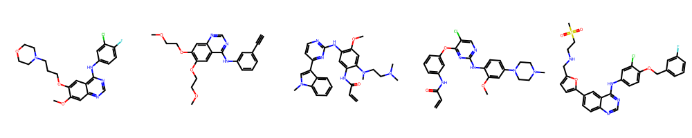
In this example (demo mode), the first molecule is gefitinib, a known FDA-approved drug against EGFR.
As a simple workaround — since we prefer to have one activity value per compound-kinase pair — we keep the value for which the compound has the best activity value, i.e., the highest pIC50 value.
[17]:
data = data.groupby(["UniprotID", "smiles"])["pIC50"].max().reset_index()
data.head()
# NBVAL_CHECK_OUTPUT
[17]:
| UniprotID | smiles | pIC50 | |
|---|---|---|---|
| 0 | P00533 | Br.CC(Nc1ncnc2[nH]c(-c3ccc(O)cc3)cc12)c1ccc(C(... | 5.336488 |
| 1 | P00533 | Br.CC(Nc1ncnc2[nH]c(-c3ccc(O)cc3)cc12)c1cccc2c... | 5.996539 |
| 2 | P00533 | Br.CC[C@@H](Nc1ncnc2[nH]c(-c3ccc(O)cc3)cc12)c1... | 8.397940 |
| 3 | P00533 | Br.C[C@@H](Nc1ncnc2[nH]c(-c3ccc(O)cc3)cc12)c1c... | 7.207608 |
| 4 | P00533 | Br.C[C@@H](Nc1ncnc2[nH]c(-c3ccc(O)cc3)cc12)c1c... | 8.420216 |
Hit or non-hit
Finally, we binarize the pIC50 values to obtain hit or non-hit using a cutoff. We use a pIC50 cutoff of \(6.3\), similarly to the cutoff used in Molecules (2021), 26(3), 629.
[18]:
cutoff = 6.3
[19]:
def binarize_pic50(pic50_value, threshold):
    """
    Binarizes a scalar value given a threshold.

    Parameters
    ----------
    pic50_value : float
        The measurement pIC50 value of a kinase-ligand pair.
    threshold : float
        The cutoff to determine activity.

    Returns
    -------
    int
        1 if the pIC50 value is above the threshold, which indicates activity.
        0 otherwise.
    """
    if pic50_value >= threshold:
        return 1
    else:
        return 0
[20]:
data["activity_binary"] = data["pIC50"].apply(binarize_pic50, args=(cutoff,))
[21]:
print(f"Current shape of data: {data.shape}")
data.head()
# NBVAL_CHECK_OUTPUT
Current shape of data: (32916, 4)
[21]:
| UniprotID | smiles | pIC50 | activity_binary | |
|---|---|---|---|---|
| 0 | P00533 | Br.CC(Nc1ncnc2[nH]c(-c3ccc(O)cc3)cc12)c1ccc(C(... | 5.336488 | 0 |
| 1 | P00533 | Br.CC(Nc1ncnc2[nH]c(-c3ccc(O)cc3)cc12)c1cccc2c... | 5.996539 | 0 |
| 2 | P00533 | Br.CC[C@@H](Nc1ncnc2[nH]c(-c3ccc(O)cc3)cc12)c1... | 8.397940 | 1 |
| 3 | P00533 | Br.C[C@@H](Nc1ncnc2[nH]c(-c3ccc(O)cc3)cc12)c1c... | 7.207608 | 1 |
| 4 | P00533 | Br.C[C@@H](Nc1ncnc2[nH]c(-c3ccc(O)cc3)cc12)c1c... | 8.420216 | 1 |
Kinase promiscuity
We now look at the kinase promiscuity.
For a given kinase, three values are computed:
the total number of measured compounds against the given kinase,
the number of active compounds against the kinase, and
the fraction of active compounds, i.e., the ratio of active compounds over the total number of measured compounds per kinase.
[22]:
def kinase_to_activity_numbers(uniprot_id, activity_df):
    """
    Retrieve the three values for a given kinase.

    Parameters
    ----------
    uniprot_id : str
        The UniProt ID of the kinase of interest, e.g. "P00533" for "EGFR".
    activity_df : pd.DataFrame
        The dataframe with activity values for kinases.

    Returns
    -------
    tuple : (int, int, float)
        The three metrics:
        1. The total number of measured compounds against the kinase.
        2. The number of active compounds against the kinase.
        3. The fraction of active compounds against the kinase.
    """
    kinase_data = activity_df[activity_df["UniprotID"] == uniprot_id]
    total_measured_compounds = len(kinase_data)
    active_compounds = len(kinase_data[kinase_data["activity_binary"] == 1])
    if total_measured_compounds > 0:
        fraction = active_compounds / total_measured_compounds
    else:
        print("No compounds were measured for this kinase.")
        fraction = np.nan
    return (total_measured_compounds, active_compounds, fraction)
Let’s see what information we get for the first kinase in our dataset:
[23]:
example_kinase = kinase_selection_df["kinase_klifs"][0]
example_uniprot = kinase_selection_df["uniprot_id"][0]

print(f"{example_kinase} ({example_uniprot}):")
example_metrics = kinase_to_activity_numbers(example_uniprot, data)
print(
    f"{'Total number of measured compounds:' : <40}"
    f"{example_metrics[0]} \n"
    f"{'Number of active compounds:' : <40}"
    f"{example_metrics[1]} \n"
    f"{'Fraction of active compounds:' : <40}"
    f"{example_metrics[2]:.2f} \n"
)
# NBVAL_CHECK_OUTPUT
EGFR (P00533):
Total number of measured compounds:     5965
Number of active compounds:             3635
Fraction of active compounds:           0.61
Let’s create a table from these values for all kinases:
[24]:
def promiscuity_table(kinase_selection, activity_df):
    """
    Create a table with all three values for all kinases.

    Parameters
    ----------
    kinase_selection : pd.DataFrame
        The DataFrame for the chosen kinases.
    activity_df : pd.DataFrame
        The DataFrame with activity values for kinases.

    Returns
    -------
    promiscuity_table : pd.DataFrame
        A DataFrame with the kinases as rows and values as columns.
    """
    promiscuity_table = pd.DataFrame(
        index=kinase_selection["kinase_klifs"], columns=["total", "actives", "fraction"]
    )
    promiscuity_table.index.name = None
    promiscuity_table.columns.name = None

    for name, uniprot_id in zip(kinase_selection["kinase_klifs"], kinase_selection["uniprot_id"]):
        values = kinase_to_activity_numbers(uniprot_id, activity_df)
        promiscuity_table.loc[name] = values
    return promiscuity_table
[25]:
kinase_promiscuity_df = promiscuity_table(kinase_selection_df, data)
kinase_promiscuity_df
# NBVAL_CHECK_OUTPUT
[25]:
| total | actives | fraction | |
|---|---|---|---|
| EGFR | 5965 | 3635 | 0.609388 |
| ErbB2 | 1700 | 1031 | 0.606471 |
| p110a | 4393 | 2827 | 0.643524 |
| KDR | 7641 | 5328 | 0.697291 |
| BRAF | 3688 | 2992 | 0.81128 |
| CDK2 | 1500 | 815 | 0.543333 |
| LCK | 1560 | 935 | 0.599359 |
| MET | 2832 | 2248 | 0.793785 |
| p38a | 3637 | 2778 | 0.763816 |
Let’s beautify the table:
[26]:
kinase_promiscuity_df.style.format("{:.3f}", subset=["fraction"]).background_gradient(
    cmap="Purples", subset=["fraction"]
).highlight_min(color="yellow", axis=None, subset=["fraction"]).highlight_max(
    color="red", subset=["fraction"]
)
[26]:
| total | actives | fraction | |
|---|---|---|---|
| EGFR | 5965 | 3635 | 0.609 |
| ErbB2 | 1700 | 1031 | 0.606 |
| p110a | 4393 | 2827 | 0.644 |
| KDR | 7641 | 5328 | 0.697 |
| BRAF | 3688 | 2992 | 0.811 |
| CDK2 | 1500 | 815 | 0.543 |
| LCK | 1560 | 935 | 0.599 |
| MET | 2832 | 2248 | 0.794 |
| p38a | 3637 | 2778 | 0.764 |
From the table, we notice that CDK2 is the least (in yellow) and BRAF the most (in red) promiscuous kinase.
Kinase similarity
We now investigate how we can use the similarity measure discussed in the Theory part to compare kinases.
[27]:
def similarity_ligand_profile(uniprot_id1, uniprot_id2, activity_df):
    """
    Compute the similarity between two kinases using ligand profiling data.

    Parameters
    ----------
    uniprot_id1 : str
        UniProt ID of first kinase of interest.
    uniprot_id2 : str
        UniProt ID of second kinase of interest.
    activity_df :  pd.DataFrame
        The DataFrame with activity values for kinases.

    Returns
    -------
    tuple : (int, int, float)
        The three metrics:
        1. The total number of measured compounds against both kinases.
        2. The number of active compounds against both kinases.
        3. The metric for kinase similarity,
                i.e. number of active compounds on both kinases
                over number of measured compounds on both kinases.
    """
    if uniprot_id1 == uniprot_id2:
        return kinase_to_activity_numbers(uniprot_id1, activity_df)
    else:
        # Data for the two kinases only
        reduced_data = activity_df[activity_df["UniprotID"].isin([uniprot_id1, uniprot_id2])]

        # Look at active compounds only
        active_entries = reduced_data[reduced_data["activity_binary"] == 1]
        # Group by compounds
        compounds = active_entries.groupby("smiles").size()
        # Look at the number of active compounds measured on both kinases
        active_compounds_on_both = compounds[compounds == 2].shape[0]

        # Look at all tested compounds
        compounds = reduced_data.groupby("smiles").size()
        # Look at the number of compounds measured on both kinases
        measured_compounds_on_both = compounds[compounds == 2].shape[0]

        if measured_compounds_on_both > 0:
            fraction = active_compounds_on_both / measured_compounds_on_both
        else:
            print(
                f"No compounds were measured on both kinases, "
                f"namely {uniprot_id1} and {uniprot_id2}."
            )
            fraction = np.nan
            measured_compounds_on_both = np.nan
            active_compounds_on_both = np.nan
        return (measured_compounds_on_both, active_compounds_on_both, fraction)
Let’s look at the values and similarity between two kinases.
[28]:
if DEMO:
    kinase1 = "EGFR"
    uniprot1 = "P00533"
    kinase2 = "MET"
    uniprot2 = "P08581"
else:
    kinase1 = kinase_selection_df["kinase_klifs"][0]
    uniprot1 = kinase_selection_df["uniprot_id"][0]
    kinase2 = kinase_selection_df["kinase_klifs"][1]
    uniprot2 = kinase_selection_df["uniprot_id"][1]

similarity_example = similarity_ligand_profile(uniprot1, uniprot2, data)
print(
    f"Values for {kinase1} and {kinase2}: \n\n"
    f"{'Total number of measured compounds:' : <50}"
    f"{similarity_example[0]} \n"
    f"{'Number of active compounds:' : <50}"
    f"{similarity_example[1]} \n"
    f"Fraction of active compounds or \n"
    f"{'ligand profile similarity:' : <50}"
    f"{similarity_example[2]:.2f} \n"
)
# NBVAL_CHECK_OUTPUT
Values for EGFR and MET:

Total number of measured compounds:               92
Number of active compounds:                       21
Fraction of active compounds or
ligand profile similarity:                        0.23
Visualize similarity as kinase matrix
Let’s first look at the non-reduced fraction of number of active compound against total number of compounds to have an idea of the counts.
[29]:
kinase_counts_matrix = pd.DataFrame(
    index=kinase_selection_df.kinase_klifs, columns=kinase_selection_df.kinase_klifs
)
kinase_counts_matrix.index.name = None
kinase_counts_matrix.columns.name = None

for i, (uniprot_id1, klifs_name1) in enumerate(
    zip(kinase_selection_df.uniprot_id, kinase_selection_df.kinase_klifs)
):
    for j, (uniprot_id2, klifs_name2) in enumerate(
        zip(kinase_selection_df.uniprot_id, kinase_selection_df.kinase_klifs)
    ):
        total, actives, _ = similarity_ligand_profile(uniprot_id1, uniprot_id2, data)
        integer_ratio = f"{actives}/{total}"
        kinase_counts_matrix.loc[klifs_name1, klifs_name2] = integer_ratio
kinase_counts_matrix
# NBVAL_CHECK_OUTPUT
No compounds were measured on both kinases, namely P04626 and P42336.
No compounds were measured on both kinases, namely P42336 and P04626.
[29]:
| EGFR | ErbB2 | p110a | KDR | BRAF | CDK2 | LCK | MET | p38a | |
|---|---|---|---|---|---|---|---|---|---|
| EGFR | 3635/5965 | 662/1170 | 13/179 | 313/893 | 27/59 | 5/40 | 31/126 | 21/92 | 18/52 |
| ErbB2 | 662/1170 | 1031/1700 | nan/nan | 72/180 | 4/16 | 4/27 | 5/33 | 1/28 | 2/16 |
| p110a | 13/179 | nan/nan | 2827/4393 | 32/174 | 1/3 | 4/12 | 0/3 | 0/1 | 0/5 |
| KDR | 313/893 | 72/180 | 32/174 | 5328/7641 | 199/262 | 71/115 | 179/413 | 184/340 | 63/122 |
| BRAF | 27/59 | 4/16 | 1/3 | 199/262 | 2992/3688 | 1/13 | 22/40 | 3/26 | 29/41 |
| CDK2 | 5/40 | 4/27 | 4/12 | 71/115 | 1/13 | 815/1500 | 2/18 | 2/22 | 1/9 |
| LCK | 31/126 | 5/33 | 0/3 | 179/413 | 22/40 | 2/18 | 935/1560 | 17/63 | 69/138 |
| MET | 21/92 | 1/28 | 0/1 | 184/340 | 3/26 | 2/22 | 17/63 | 2248/2832 | 1/20 |
| p38a | 18/52 | 2/16 | 0/5 | 63/122 | 29/41 | 1/9 | 69/138 | 1/20 | 2778/3637 |
Note that the total number of tested compounds as well as the number of active compounds on two kinases vary largely.
For the p110a-ErbB2 pair, there are none.
For p110a and [BRAF, CDK2, LCK, MET and p38a], there are less than \(13\) commonly tested compounds.
In contrast, the EGFR-ErbB2 pair has \(1170\) commonly tested compounds, of which \(662\) were active on both.
Now let’s look at the similarity, in this case, the reduced fraction:
[30]:
kinase_similarity_matrix = np.zeros((len(kinase_selection_df), len(kinase_selection_df)))
for i, uniprot_id1 in enumerate(kinase_selection_df.uniprot_id):
    for j, uniprot_id2 in enumerate(kinase_selection_df.uniprot_id):
        kinase_similarity_matrix[i, j] = similarity_ligand_profile(uniprot_id1, uniprot_id2, data)[
            2
        ]
No compounds were measured on both kinases, namely P04626 and P42336.
No compounds were measured on both kinases, namely P42336 and P04626.
[31]:
kinase_similarity_matrix_df = pd.DataFrame(
    data=kinase_similarity_matrix,
    index=kinase_selection_df.kinase_klifs,
    columns=kinase_selection_df.kinase_klifs,
)
kinase_similarity_matrix_df.index.name = None
kinase_similarity_matrix_df.columns.name = None
kinase_similarity_matrix_df
# NBVAL_CHECK_OUTPUT
[31]:
| EGFR | ErbB2 | p110a | KDR | BRAF | CDK2 | LCK | MET | p38a | |
|---|---|---|---|---|---|---|---|---|---|
| EGFR | 0.609388 | 0.565812 | 0.072626 | 0.350504 | 0.457627 | 0.125000 | 0.246032 | 0.228261 | 0.346154 |
| ErbB2 | 0.565812 | 0.606471 | NaN | 0.400000 | 0.250000 | 0.148148 | 0.151515 | 0.035714 | 0.125000 |
| p110a | 0.072626 | NaN | 0.643524 | 0.183908 | 0.333333 | 0.333333 | 0.000000 | 0.000000 | 0.000000 |
| KDR | 0.350504 | 0.400000 | 0.183908 | 0.697291 | 0.759542 | 0.617391 | 0.433414 | 0.541176 | 0.516393 |
| BRAF | 0.457627 | 0.250000 | 0.333333 | 0.759542 | 0.811280 | 0.076923 | 0.550000 | 0.115385 | 0.707317 |
| CDK2 | 0.125000 | 0.148148 | 0.333333 | 0.617391 | 0.076923 | 0.543333 | 0.111111 | 0.090909 | 0.111111 |
| LCK | 0.246032 | 0.151515 | 0.000000 | 0.433414 | 0.550000 | 0.111111 | 0.599359 | 0.269841 | 0.500000 |
| MET | 0.228261 | 0.035714 | 0.000000 | 0.541176 | 0.115385 | 0.090909 | 0.269841 | 0.793785 | 0.050000 |
| p38a | 0.346154 | 0.125000 | 0.000000 | 0.516393 | 0.707317 | 0.111111 | 0.500000 | 0.050000 | 0.763816 |
[32]:
# Show matrix with background gradient
cm = sns.light_palette("green", as_cmap=True)
kinase_similarity_matrix_df.style.background_gradient(cmap=cm).format("{:.3f}")
[32]:
| EGFR | ErbB2 | p110a | KDR | BRAF | CDK2 | LCK | MET | p38a | |
|---|---|---|---|---|---|---|---|---|---|
| EGFR | 0.609 | 0.566 | 0.073 | 0.351 | 0.458 | 0.125 | 0.246 | 0.228 | 0.346 |
| ErbB2 | 0.566 | 0.606 | nan | 0.400 | 0.250 | 0.148 | 0.152 | 0.036 | 0.125 |
| p110a | 0.073 | nan | 0.644 | 0.184 | 0.333 | 0.333 | 0.000 | 0.000 | 0.000 |
| KDR | 0.351 | 0.400 | 0.184 | 0.697 | 0.760 | 0.617 | 0.433 | 0.541 | 0.516 |
| BRAF | 0.458 | 0.250 | 0.333 | 0.760 | 0.811 | 0.077 | 0.550 | 0.115 | 0.707 |
| CDK2 | 0.125 | 0.148 | 0.333 | 0.617 | 0.077 | 0.543 | 0.111 | 0.091 | 0.111 |
| LCK | 0.246 | 0.152 | 0.000 | 0.433 | 0.550 | 0.111 | 0.599 | 0.270 | 0.500 |
| MET | 0.228 | 0.036 | 0.000 | 0.541 | 0.115 | 0.091 | 0.270 | 0.794 | 0.050 |
| p38a | 0.346 | 0.125 | 0.000 | 0.516 | 0.707 | 0.111 | 0.500 | 0.050 | 0.764 |
Note that the diagonal contains the previously discussed promiscuity values.
As mentioned above, no compounds were measured on both ErbB2 and p110a and therefore creates a np.nan entry which can be problematic for algorithmic reason.
As a simple workaround, we will fill the NA values with zero.
[33]:
kinase_similarity_matrix_df = kinase_similarity_matrix_df.fillna(0)

kinase_similarity_matrix_df.style.background_gradient(cmap=cm).format("{:.3f}")
[33]:
| EGFR | ErbB2 | p110a | KDR | BRAF | CDK2 | LCK | MET | p38a | |
|---|---|---|---|---|---|---|---|---|---|
| EGFR | 0.609 | 0.566 | 0.073 | 0.351 | 0.458 | 0.125 | 0.246 | 0.228 | 0.346 |
| ErbB2 | 0.566 | 0.606 | 0.000 | 0.400 | 0.250 | 0.148 | 0.152 | 0.036 | 0.125 |
| p110a | 0.073 | 0.000 | 0.644 | 0.184 | 0.333 | 0.333 | 0.000 | 0.000 | 0.000 |
| KDR | 0.351 | 0.400 | 0.184 | 0.697 | 0.760 | 0.617 | 0.433 | 0.541 | 0.516 |
| BRAF | 0.458 | 0.250 | 0.333 | 0.760 | 0.811 | 0.077 | 0.550 | 0.115 | 0.707 |
| CDK2 | 0.125 | 0.148 | 0.333 | 0.617 | 0.077 | 0.543 | 0.111 | 0.091 | 0.111 |
| LCK | 0.246 | 0.152 | 0.000 | 0.433 | 0.550 | 0.111 | 0.599 | 0.270 | 0.500 |
| MET | 0.228 | 0.036 | 0.000 | 0.541 | 0.115 | 0.091 | 0.270 | 0.794 | 0.050 |
| p38a | 0.346 | 0.125 | 0.000 | 0.516 | 0.707 | 0.111 | 0.500 | 0.050 | 0.764 |
Save kinase similarity matrix
[34]:
kinase_similarity_matrix_df.to_csv(DATA / "kinase_similarity_matrix.csv")
Kinase distance matrix
The similarity matrix \(SM\) is converted to a pseudo-distance matrix (all entries of the similarity matrix are between \(0\) and \(1\)):
[35]:
print(
    f"The values of the similarity matrix lie between: "
    f"{kinase_similarity_matrix_df.min().min():.2f}"
    f" and {kinase_similarity_matrix_df.max().max():.2f}"
)
# NBVAL_CHECK_OUTPUT
The values of the similarity matrix lie between: 0.00 and 0.81
[36]:
kinase_distance_matrix_df = 1 - kinase_similarity_matrix_df
Finally, we set the diagonal values to \(0\) and we obtain the kinase distance matrix:
[37]:
# np.fill_diagonal(kinase_distance_matrix_df.values, 0) # read-only error
# safe assignment
for i in range(len(kinase_distance_matrix_df)):
    kinase_distance_matrix_df.iloc[i, i] = 0
[38]:
kinase_distance_matrix_df.style.background_gradient(cmap=cm).format("{:.3f}")
[38]:
| EGFR | ErbB2 | p110a | KDR | BRAF | CDK2 | LCK | MET | p38a | |
|---|---|---|---|---|---|---|---|---|---|
| EGFR | 0.000 | 0.434 | 0.927 | 0.649 | 0.542 | 0.875 | 0.754 | 0.772 | 0.654 |
| ErbB2 | 0.434 | 0.000 | 1.000 | 0.600 | 0.750 | 0.852 | 0.848 | 0.964 | 0.875 |
| p110a | 0.927 | 1.000 | 0.000 | 0.816 | 0.667 | 0.667 | 1.000 | 1.000 | 1.000 |
| KDR | 0.649 | 0.600 | 0.816 | 0.000 | 0.240 | 0.383 | 0.567 | 0.459 | 0.484 |
| BRAF | 0.542 | 0.750 | 0.667 | 0.240 | 0.000 | 0.923 | 0.450 | 0.885 | 0.293 |
| CDK2 | 0.875 | 0.852 | 0.667 | 0.383 | 0.923 | 0.000 | 0.889 | 0.909 | 0.889 |
| LCK | 0.754 | 0.848 | 1.000 | 0.567 | 0.450 | 0.889 | 0.000 | 0.730 | 0.500 |
| MET | 0.772 | 0.964 | 1.000 | 0.459 | 0.885 | 0.909 | 0.730 | 0.000 | 0.950 |
| p38a | 0.654 | 0.875 | 1.000 | 0.484 | 0.293 | 0.889 | 0.500 | 0.950 | 0.000 |
Save kinase distance matrix
[39]:
kinase_distance_matrix_df.to_csv(DATA / "kinase_distance_matrix.csv")
Discussion
In this talktorial, we investigate how activity data can be used as a measure of similarity between kinases. The fraction of compounds tested as actives over the total number of measured compounds is a way of accessing the similarity. Moreover, using the same rationale, the promiscuity of a kinase can be quantified using the ratio of active compounds over measured compounds.
When working with these data, we have to keep in mind that some kinases have much higher coverage with respect to the number of compounds that were tested against them, leading to an imbalance in information content. This cannot be inferred from the calculated fraction. For example, the pairs EGFR-KDR and EGFR-p38a both have a profile similarity of \(0.35\). However, the first was calculated based on \(893\) tested compounds, whereas the latter on \(52\) only.
The kinase distance matrix above will be reloaded in Talktorial T028, where we compare kinase similarities from different perspectives, including the ligand profile perspective we have talked about in this talktorial.
Quiz
Is there an optimal way to deal with multiple kinase-ligand measurements?
Can promiscuity be fairly compared between two kinases if one has been tested against many compounds whereas the other only against very few?
Using the similarity described in this talktorial, what does it mean that two kinases have a similarity of \(0\), as is the case for p110a and LCK?