T017 · Advanced NGLview usage
Note: This talktorial is a part of TeachOpenCADD, a platform that aims to teach domain-specific skills and to provide pipeline templates as starting points for research projects.
Authors:
Jaime Rodríguez-Guerra, 2021, Volkamer lab, Charité
Dominique Sydow, 2021, Volkamer lab, Charité
Aim of this talktorial
NGLView is a powerful Jupyter widget that allows you to show molecular structures in your notebooks in a 3D interactive view! It supports both single conformations and trajectories, as well as a plethora of representations. In this talktorial we will cover how to use it in different scenarios, from simpler cases to more intricate ones.
Contents in Theory
NGL and NGLView
NGL object model and terminology
Contents in Practical
First steps: make sure everything works!
Experiment with the interactive controls
Basic API usage:
Show a structure using its PDB identifier
Show a structure using a local file
Saving the widget state as a screenshot for offline viewing
Customize the representations
Control representations by selections
NMR and multimodel structures
Load more than one structure
Show and hide components
Advanced usage:
Custom coloring schemes and representations
Add geometric objects at selected atoms
Create interactive interfaces
Access the JavaScript layer
Troubleshooting tips:
Check which Jupyter platform you are working from
How to install
nglview, the right way
References
NGL manuscript: Rose et al., Nucl Acids Res. (2015), 43 (W1), W576-W579 (https://academic.oup.com/nar/article/43/W1/W576/2467902)
NGLView manuscript: Nguyen et al., Bioinformatics (2018), 34 (7), 1241-1242 (https://academic.oup.com/bioinformatics/article/34/7/1241/4721781)
NGLView Q&A issues. A lot of hidden knowledge in these conversations!
[1]:
import sys
if "google.colab" in sys.modules:
%pip install teachopencadd --no-deps -q
!teachopencadd -d 17
%pip uninstall teachopencadd -y -q
%pip install -qr requirements.txt
Theory
NGL and NGLView
NGL is a WebGL-accelerated JavaScript library for the depiction of 3D macromolecular structures on your browser. It doesn’t require any software installation! It has been widely adopted in the data science community, partially thanks to the NGLView integrations in the Jupyter ecosystem. While tightly connected, NGL and NGLView are two separate projects and understanding this difference is key.
NGL is the JavaScript library that renders the molecular structures in your browser using WebGL. It can be embedded in any webpage, see the demo application.
NGLView wraps NGL so it can be used from a Jupyter notebook running a Python kernel. This is possible thanks to the integrations provided by the IPyWidgets project.
When you import nglview, you are loading a Python package that knows how to talk to the underlying JavaScript library. The process of telling nglview which structure you want to see involves more steps than you may think!
Importing the package:
import nglviewonly loadsnglviewPython package. This is usually provided bycondaorpip.The Python package must now find the JavaScript components. These are bundled as part of the Python package data files, but they need to be placed in the right location so the browser can load them in the Jupyter UI.
Importing the Python package successfully does not necessarily imply that the JavaScript layer was loaded correctly! Note: This is a common error and we have covered some troubleshooting at the end of the talktorial.
Showing a 3D structure:
When you ask for a PDB ID to be shown, NGLView will pass NGL the URL of the file you want to download (we’ll use a sepertate function to download the PDB file safely and then pass it to NGLView). Then, the JavaScript layer takes over and downloads the contents to your browser’s memory, creates JavaScript objects for the macromolecular structure and then renders it in a WebGL-enabled
<canvas>HTML5 element.If you want to open a local file, you can either:
Open the file with Python and pass the contents of the file to NGL.
Pass the location of the file in disk to NGLView, which will transform it to a download link that NGL (being JavaScript) can use to get access to the file. Note: This step is fragile and can break with different package versions, so we recommend opening the file in Python first. An example is provided later!
If you want to view a molecular object as provided by a Python library (RDKit, BioPython, MDAnalysis…), NGLView will try to recognize the object model and convert it to a suitable format for NGL (usually a PDB string). This happens transparently through some helper functions.
Given the complexity of these interactions, you must understand that NGLView only provides a Python interface to the most common features provided by NGL. Some of its advanced features are not exposed directly, but the good news is that you can always send code snippets to the underlying JavaScript objects.
We will cover all of these subtleties with different examples through this talktorial.
NGL object model and terminology
When you ask for a 3D viewer, NGLView (the Python package) will create an object called NGLWidget, which wraps the NGL Stage JavaScript object in an IPyWidget object. NGLWidget acts as the bridge between Python and JavaScript. When you autocomplete on a view instance, you are exploring the NGLWidget Python attributes and methods.
Once you are in JavaScript territory, you are handling the NGL object model. This basically consists of the Stage, which can host one or more components. A component can be a molecular structure or a geometric shape. Components can be rendered with one or more representations. For example, when you see a protein ligand complex (like, let’s say, PDB ID 3PK2), you are seeing:
The NGL
Stage, the interactive canvasA single component, the in-memory JavaScript object for 3PK2. Take into account that a component can store more than one molecule or model in the physical sense!
Two representations: ribbon for the backbone, ball and stick for the ligand
If you want to see the water molecules too, you would add one more representation targeting only the solvent.
Representations do not only include how the structure looks like. The NGL implementation also considers some types of measurements as representations. If you want to see the van der Waals surface, that’s a representation in NGL terms. Measuring the distance between two atoms and displaying that as a pointed line, that’s a representation too. Labels count as representations, too.
However, if you want to add a shape that points to an arbitrary spot in your protein, that’s a shape, which is a subtype of a component!
Confusing? One way to remember the difference: representations depend on the coordinates provided by a component. They don’t have coordinates or their own! Shapes, being able to be placed in arbitrary places, are not representations, but components on their own.
To make sure you got the gist, you can also check the examples in the demo application (dropdown in the top menu) and get more familiar with the NGL terminology. Each example will load a state on the 3D canvas, with components being on the top level of the hierarchy, and their representations under each one.
This should cover the core concepts at the theory level, but this won’t make much sense until you see it in action so… let’s go!
Practical
Note: Since NGLView is an interactive widget, most of the features discussed in this talktorial will be best enjoyed in a running Jupyter environment. If you are reading this from the online static preview, you are missing out a lot of cool things!
[2]:
from pathlib import Path
HERE = Path(_dh[-1])
DATA = HERE / "data"
First steps: make sure everything works!
[3]:
import nglview as nv
from pypdb.clients.pdb.pdb_client import get_pdb_file
nv.demo()
If you don’t see a 3D interactive view of protein in the output of the cell above, check the Troubleshooting tips section at the end of this notebook.
Experiment with the interactive controls
The view above is interactive! You can use your mouse to:
Translation: right click + drag
Rotation: left click + drag
Z-axis rotation: Ctrl + right click + drag
Zoom: scroll wheel
Center view: left click on the desired atom (or its representation)
You can also represent distances, angles and dihedrals by following this procedure:
Right click on a single atom. You’ll see a green sphere wrapping it.
Right click on another atom. You’ll see now two green spheres. You can add up to four atoms to a selection this way (including the first one)
Right click again on the last atom you selected to finalize the operation.
If you picked two atoms, you’ll see a dashed line between the two atoms, along with the reported distance in Å.
If you picked three atoms, you’ll see a circular sector with the angle reported in degrees (°).
If you picked four atoms, you’ll see a circular sector with the dihedral angle reported in degrees (°).
To remove a distance/angle/dihedral representation, repeat the sequence on the same atoms.
Figure: Step by step procedure to represent geometric measurements in NGLView.
Basic API usage
nglview wraps the ngl.js JavaScript library with an IPyWidget subclass named NGLWidget. You can create widget objects using the class directly:
viewer = nv.NGLWidget()
But for simple cases, it’s more convenient to use the nv.show_* helper functions. This is the current list of functions available:
[4]:
print("NGLView version:", nv.__version__)
for attr in dir(nv):
if attr.startswith("show_"):
print(f" nv.{attr}(...)")
NGLView version: 4.0
nv.show_ase(...)
nv.show_asetraj(...)
nv.show_biopython(...)
nv.show_file(...)
nv.show_htmd(...)
nv.show_iodata(...)
nv.show_iotbx(...)
nv.show_mdanalysis(...)
nv.show_mdtraj(...)
nv.show_openbabel(...)
nv.show_parmed(...)
nv.show_pdbid(...)
nv.show_prody(...)
nv.show_psi4(...)
nv.show_pymatgen(...)
nv.show_pytraj(...)
nv.show_qcelemental(...)
nv.show_rdkit(...)
nv.show_rosetta(...)
nv.show_schrodinger(...)
nv.show_simpletraj(...)
nv.show_structure_file(...)
nv.show_text(...)
nv.show_url(...)
Note how it has functions for:
local files (different file formats are supported out of the box, check the list here)
online resources (PDB IDs, URLs…)
objects from popular libraries (BioPython, MDAnalysis, RDKit…). This includes both single structures and trajectories! You can see it in action in Talktorial T020, a talktorial on analyzing molecular dynamics simulations.
Show a structure using its PDB identifier
For now, nv.show_pdbid isn’t working so we substitute the process using get_pdb_nglviewer function.
Use pypdb.get_pdb_file to fetch a PDB structure from the RCSB PDB website and display using nv.show_file:
[5]:
def get_structure(pdb_id):
# download the PDB file content.
pdb_file_content = get_pdb_file(pdb_id)
# create an nglview structure object from the content
structure = nv.TextStructure(pdb_file_content, ext="pdb")
return structure
def get_pdb_nglviewer(pdb_id, default_representation=True, gui=False):
structure = get_structure(pdb_id)
# set structure viewer
nglviewer = nv.show_file(structure, default_representation=default_representation, gui=gui)
return nglviewer
[6]:
# nv.show_pdbid("3pk2")
get_pdb_nglviewer("3pk2")
Sending GET request to https://files.rcsb.org/download/3pk2.pdb to fetch 3pk2's pdb file as a string.
Show a structure using a local file
In other cases, you will have a local file produced by other parts of your pipeline. To load local files, you would need to use nv.show_file("path/to/local/file.pdb"). If you are using Jupyter Notebook as the UI, this will work out of the box.
However, the Jupyter ecosystem is moving towards Lab, where things work a bit differently. One of them is accessing local files. This is a known issue, so we are going to provide a workaround until this is fixed. The trick consists of opening the file with Python first, and then passing the handler to NGLView, instead of the path. You also need to specify the extension for that file handler (pdb in this example). display(...) is
needed to explicitly export the widget view to the output because we are inside the open() context manager.
[7]:
with open(DATA / "1ARM.pdb") as f:
display(nv.show_file(f, ext="pdb"))
You can also save the widget returned by the function (view, by convention) and evaluate it at the global level:
[8]:
with open(DATA / "1ARM.pdb") as f:
view = nv.show_file(f, ext="pdb")
view
This has the advantage of allowing you to modify the state of the widget from the Python interface, as you will see in the next steps.
Saving the widget state as a screenshot for offline viewing
In some cases, you might want to take a screenshot of the current state of the widget (e.g. to save a static preview). This is a step that necessarily involves three separate cells. Although it is very tempting to merge all the cells together, it will not work unless each cell is run separately:
viewwill show the widget output. You can use your mouse to move it to a nice orientation, if you want.view.render_image(...)will export the current canvas contents from the JavaScript layer to the Python layer. This is the “screenshot” moment.view._display_image()will export the contents of the Python layer to the cell output.
[9]:
view
Let’s render an image of this view with the following parameters:
trim=Trueremoves the blank padding around the moleculefactor=2asks for a 2x resolution render for higher quality, but not too much (default is 4x)
[10]:
view.render_image(trim=True, factor=2)
[10]:
[11]:
view._display_image()
[11]:
Customize the representations
You can add more representations using the view.add_* methods. The following ones are available. Take into account that in NGL, a representation can include visual tools other than how a protein or ligand is depicted. For example, calculating (and showing) distance measurements is also a representation. We will talk more about this later, but you can also check this part of the NGL documentation.
Note that some
.add_*functionalities actually are convenience methods to add more components to the canvas, not representations! This is the case withadd_component,add_pdbid,add_structureandadd_trajectory, among others.
[12]:
for attr in dir(view):
if attr.startswith("add_"):
print(f"view.{attr}(...)")
view.add_axes(...)
view.add_backbone(...)
view.add_ball_and_stick(...)
view.add_cartoon(...)
view.add_class(...)
view.add_component(...)
view.add_contact(...)
view.add_distance(...)
view.add_helixorient(...)
view.add_hyperball(...)
view.add_label(...)
view.add_licorice(...)
view.add_line(...)
view.add_pdbid(...)
view.add_point(...)
view.add_principal_axes(...)
view.add_representation(...)
view.add_ribbon(...)
view.add_rocket(...)
view.add_rope(...)
view.add_simplified_base(...)
view.add_slice(...)
view.add_spacefill(...)
view.add_structure(...)
view.add_surface(...)
view.add_trace(...)
view.add_traits(...)
view.add_trajectory(...)
view.add_tube(...)
view.add_unitcell(...)
Note that each representation type admits arbitrary keyword arguments that are not documented in the Python layer. Refer to the JavaScript documentation to see how you can customize each one. See the *RepresentationParameters objects here.
Tip: Use Ctrl+F to find for the correct entry in the table of contents on the left!
Another way to find the options is to look at the *Representation constructor method. For example, if you want to add a ball and stick representation, you will need the add_ball_and_stick method. Search for ballandstick and you will arrive to the JavaScript class BallAndStickRepresentation here. You will see the params attribute in the constructor
docstring, which will take you to the table of options you can use (see here):
sphereDetailradialSegmentsopenEndeddisableImpostoraspectRatiolineOnlylinewidthcylinderOnlymultipleBondbondSpacingbondScale
Unfortunately, some representations are not fully documented, so you might even need to dive in to the JavaScript source… at that point, you might want to ask for help in their GitHub repository!
Control representations by selections
If you combine all those add_* functions with NGL’s powerful selection language you can adapt the style of your structures to your liking. This is specially useful when you disable the default representation to start from scratch.
For this example, we will use 3PK2, a streptavidin binded to a biotine derivative that is coordinated to a transition metal ion (Iridium). For details see 4IR. This is considered an artificial metalloenzyme, how cool is that?!
[13]:
# view = nv.show_pdbid("3pk2", default_representation=False)
view = get_pdb_nglviewer("3pk2", default_representation=False)
view
Sending GET request to https://files.rcsb.org/download/3pk2.pdb to fetch 3pk2's pdb file as a string.
The above widget is now completely blank*. That doesn’t mean the structures were not loaded (the components are loaded but no representation is set, yet). Then, we have to add representations. Look how the widget updates over the next steps (including in the view above).
* If the widget is not black, you may have executed the whole talktorial at once; please restart and execute the talktorial cell by cell.
[14]:
# add ribbon to protein only
view.add_cartoon("protein")
view
Now we want to ask the JS backend to render the current state of the widget to an internal image buffer with .render_image. We will use this to depict the progressive changes to the representation over the next cells.
[15]:
view.render_image(trim=True, factor=2);
Once rendered, we can show the screenshot in the notebook!
[16]:
view._display_image()
[16]:
By default, the camera is not centered on the molecule, but we can remediate that with .center()
[17]:
view.center()
view.render_image(trim=True, factor=2);
[18]:
view._display_image()
[18]:
Didn’t we say we had a super cool ligand? Where is it? Hm, let’s add a ball & stick representation for it!
[19]:
view.add_ball_and_stick("ligand")
view.render_image(trim=True, factor=2);
[20]:
view._display_image()
[20]:
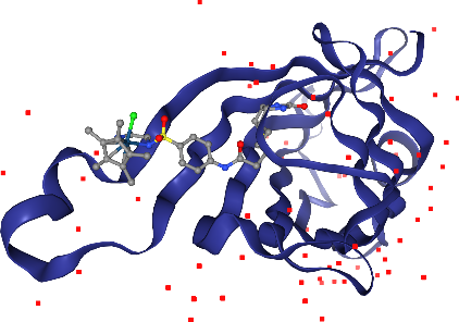
Crystallographic waters should be displayed, but in a subtle way that does not get in the way. line representations work nice for this. Note: Crystallographic waters consist of an oxygen atom only since hydrogen atoms are not resolved by X-ray crystallography, so we see dots instead of lines.
[21]:
view.add_line("water")
view.render_image(trim=True, factor=2);
[22]:
view._display_image()
[22]:

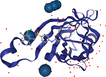
Oh, we almost forgot about the Iridium ion. Where is it? We better highlight it so we don’t miss it. We can ask for a larger sphere style if we use spacefill for that atom only. We can select by elements using _ in front of the element symbol.
[23]:
view.add_spacefill("_Ir")
view.render_image(trim=True, factor=2);
[24]:
view._display_image()
[24]:
Wait, in addition to the ligand Iridium, we can see more in other parts of the solvent? Hm, we don’t want to see those, since they are probably artifacts of the X-ray preparation. Let’s undo the last step with the corresponding .remove_*() method.
[25]:
view.remove_spacefill()
view.render_image(trim=True, factor=2);
[26]:
view._display_image()
[26]:
Now, let’s add spacefill again, but only for the Iridium ion in the ligand. The selection query needs to satisfy atoms that are both Iridium and part of the ligand.
[27]:
view.add_spacefill("ligand and _Ir")
view.render_image(trim=True, factor=2);
[28]:
view._display_image()
[28]:
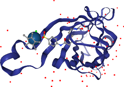
Perfect!
NMR and multimodel structures
If you are dealing with NMR structures or multimodel PDBs, there will be multiple conformations. By default, only the first one will be loaded:
[29]:
# By default, first model only
# nv.show_pdbid("1rfo")
get_pdb_nglviewer("1rfo")
Sending GET request to https://files.rcsb.org/download/1rfo.pdb to fetch 1rfo's pdb file as a string.
To display all of them, you need to disable the default representation and provide your own:
[30]:
# all models require custom representation
view = get_pdb_nglviewer("1rfo", default_representation=False)
view.center()
view.add_cartoon()
view
Sending GET request to https://files.rcsb.org/download/1rfo.pdb to fetch 1rfo's pdb file as a string.
Load more than one structure
Once you have the view instance around, you can start doing more advanced stuff with NGLView! For example, loading more than one structure!
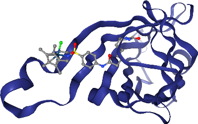
Let’s start with some depictions of Bos taurus’ carboxypeptidase. The RCSB PDB contains several structures for this enzyme. We can choose two of them that are very similar, except for a little difference. That way, if we load both on NGLView and show/hide one at a time, we will be able to spot the differences right away!
1YME: Structure of carboxypeptidase, which features a Zn ion
1ARM: Same structure, but the Zn has been replaced with a Hg ion
[31]:
view = get_pdb_nglviewer("1YME")
view
Sending GET request to https://files.rcsb.org/download/1YME.pdb to fetch 1YME's pdb file as a string.
Now, let’s add 1ARM, which contains a ligand TRS. Note that the view above will get updated automatically:
[32]:
# view.add_component(nv.PdbIdStructure("1ARM"))
view.add_component(get_structure("1ARM"))
Sending GET request to https://files.rcsb.org/download/1ARM.pdb to fetch 1ARM's pdb file as a string.
[32]:
<nglview.component.ComponentViewer at 0x116703ef0>
view contains now two components, as shown in:
[33]:
view.n_components
[33]:
2
The individual components are available via view.component_{index} or view[{index}]:
[34]:
view[0]
[34]:
<nglview.component.ComponentViewer at 0x11677be90>
[35]:
view.component_0
[35]:
<nglview.component.ComponentViewer at 0x1167033b0>
Show and hide components
Since each component can control their own representations, we can hide some parts on command using the .hide(). This action is undone with .show().
[36]:
view[1].hide()
Note how the TRS ligand disappeared from the view above. Now, let’s show it again:
[37]:
view[1].show()
If you don’t want to keep scrolling up to see the changes, you can also create a new output view, if you are using Jupyter Lab. To do that, right-click in the left margin of the input cell above (the one with view) and select the following option. Note that you can drag that tile around to compose complex interfaces!

Advanced usage
Custom coloring schemes and representations
In addition to different kinds of representations, you can also alter how each part of the displayed structure is colored. So far we have only used the default coloring, but NGL provides several default schemes (check this list and also nv.color.COLOR_SCHEMES). The color schemes - and also names - can be used as arguments of a given representation.
[38]:
print(nv.color.COLOR_SCHEMES)
[' ', 'picking', 'random', 'uniform', 'atomindex', 'residueindex', 'chainindex', 'modelindex', 'sstruc', 'element', 'resname', 'bfactor', 'hydrophobicity', 'value', 'volume', 'occupancy']
[39]:
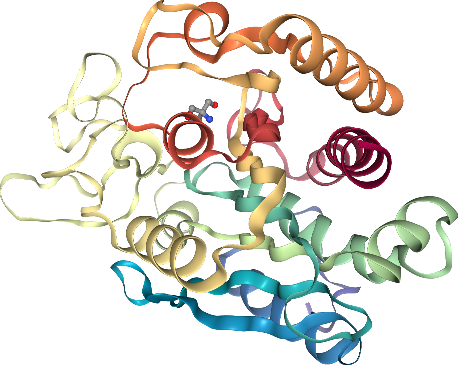
view = get_pdb_nglviewer("1PIE", default_representation=False)
view.add_ribbon("protein", color_scheme="sstruc") # color based on secondary structure
view.add_ball_and_stick("ligand")
view.center()
view
Sending GET request to https://files.rcsb.org/download/1PIE.pdb to fetch 1PIE's pdb file as a string.
You can show all side chains by applying the licorice scheme on the selection sidechainAttached directly (check the selection query docs for more detail, e.g. sidechainAttached = “Select the side-chain and C-alpha atoms plus the backbone nitrogen in case of proline.”).
Note that you can also ignore coloring schemes and use a color directly. The color option supports any of these notations:
Named colors like
redorblue, but always lowercase! Check the full list of named CSS colors.Hexadecimal strings following the CSS notation. For example, yellow is encoded as
"#FFFF00".Hexadecimal integers. In this notation, yellow is encoded as
0xFFFF00.
[40]:
view.add_licorice(
"sidechainAttached ", color="red"
) # color="#FF0000" or color=0xFF0000 would also work!
What if you need a coloring scheme not available as a keyword? You can build it via two functions in nglview.color.ColormakerRegistry:
nv.color.ColormakerRegistry.add_selection_schemeexpects ascheme_id(astrwith some name of your choice) plus a list of two-element sublists. Each sublist must define:First element (
str): the color name or coloring scheme to be appliedSecond element (
str): a selection query this color or scheme will be applied to
nv.color.ColormakerRegistry.add_scheme_funcexpects ascheme_id(astrwith some name of your choice) plus anotherstrobject that defines a JavaScript function that takes NGL atoms.
These examples are taken directly from the corresponding docstrings:
[41]:
# residues from 1 to 100 will be blue; 101 to 1000 will be red
nv.color.ColormakerRegistry.add_selection_scheme(
"my_custom_scheme", [["blue", "1-100"], ["red", "101-1000"]]
)
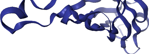
view = get_pdb_nglviewer("1EYE", default_representation=False)
view.add_cartoon(color="my_custom_scheme")
view.center()
view
Sending GET request to https://files.rcsb.org/download/1EYE.pdb to fetch 1EYE's pdb file as a string.
You can build the list of sublists programmatically for more complex visualizations. Check this external notebook for an example!
[42]:
js_function = """
this.atomColor = function (atom) {
if (atom.serial < 500) {
return 0x0000FF // blue
} else if (atom.serial < 1000) {
return 0xFF0000 // red
} else {
return 0x00FF00 // green
}
}
"""
nv.color.ColormakerRegistry.add_scheme_func("awesome", js_function)
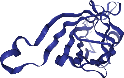
view = get_pdb_nglviewer("1EYE", default_representation=False)
view.center()
view.add_cartoon(color="awesome")
view
Sending GET request to https://files.rcsb.org/download/1EYE.pdb to fetch 1EYE's pdb file as a string.
Add geometric objects at selected atoms
For some figures, it’s often useful to mark certain areas of your structure with geometric or textual annotations. This functionality is available under a mixture of representation styles and nglview.shape functions.
[43]:
view = get_pdb_nglviewer("1YES")
view
Sending GET request to https://files.rcsb.org/download/1YES.pdb to fetch 1YES's pdb file as a string.
[44]:
# Add volume for residues 0-50
view.add_surface("0-50")
Let’s measure the distance between GLU223 and GLU200 view.add_distance takes a list of sublists. The sublists must contain atom indices (int) or a selection query that returns exactly one atom (in this case alpha carbon for residues 223 and 200). Don’t forget the black label color or you won’t see the distance value (default is white).
[45]:
view.add_distance(atom_pair=[["223.CA", "200.CA"]], label_color="black")
Now we want to add a sphere next to ILE 151… The function is view.shape.add_sphere(..):
[46]:
view.shape.add_sphere
[46]:
<bound method Shape._make_func.<locals>.make_func.<locals>.func of <nglview.shape.Shape object at 0x1167c33e0>>
But it takes XYZ coordinates. How do we get access to that information? When you click on a residue or atom, you’ll see that the top left corner of the widget exposes some details. We clicked on ILE151, and it printed ATOM: [ILE]151:A.CA. That means that the alpha carbon of residue 151 in chain A is selected. The best part is that this information is exposed to Python via view.picked!
Go and select ILE151 before executing the next cell!
[47]:
view.picked
[47]:
{}
The coordinates are hence view.picked["atom1"]["x"], view.picked["atom1"]["y"], view.picked["atom1"]["z"]:
[48]:
if "atom1" in view.picked:
sphere = view.shape.add_sphere(
[view.picked["atom1"]["x"], view.picked["atom1"]["y"], view.picked["atom1"]["z"]],
[0.5, 0.5, 0.5],
10,
"gray sphere with 10A radius",
)
To change the opacity of the sphere you will need to work with .update_representation and the component indices. It’s a bit involved, but this is how you have to do it:
[49]:
# The sphere is the last thing we added, so the component index is the last one (n_components - 1)
view.update_representation(component=view.n_components - 1, opacity=0.5)
Create interactive interfaces
One of the secret features of NGLView is the interactive GUI! Enabling it is surprisingly easy and will give you some extra control on the representations.
There are two GUIs included:
The default (
gui=True), which uses IPyWidgetsThe one NGL uses in their demo app
[50]:
# This is the default one
get_pdb_nglviewer("1RFO", gui=True)
Sending GET request to https://files.rcsb.org/download/1RFO.pdb to fetch 1RFO's pdb file as a string.
Now bring in the NGL GUI. Sometimes the canvas itself does not load, so try to execute it twice. See discussion here for more details.
[51]:
view = get_pdb_nglviewer("1RFO")
# Uncomment the lines below
# view.gui_style = "NGL"
# view
Sending GET request to https://files.rcsb.org/download/1RFO.pdb to fetch 1RFO's pdb file as a string.
Since the NGL GUI currently causes artifacts when rendered as HTML (see this issue), we only show below a screenshot of the NGL GUI. If you are working with this notebook in an executable mode, do uncomment the lines in the cell above and rerun the cell to load the NGL GUI.
Customize your own GUI with IPyWidgets
Since nglview exposes NGL as an IPython/Jupyter widget, it can be used to compose advanced dashboards in combination with the IPyWidgets project.
For example, a simple model picker for multimodel structures like in NMR studies (multimodel structure = multiple sets of coordinates for the same structure in one PDB file).
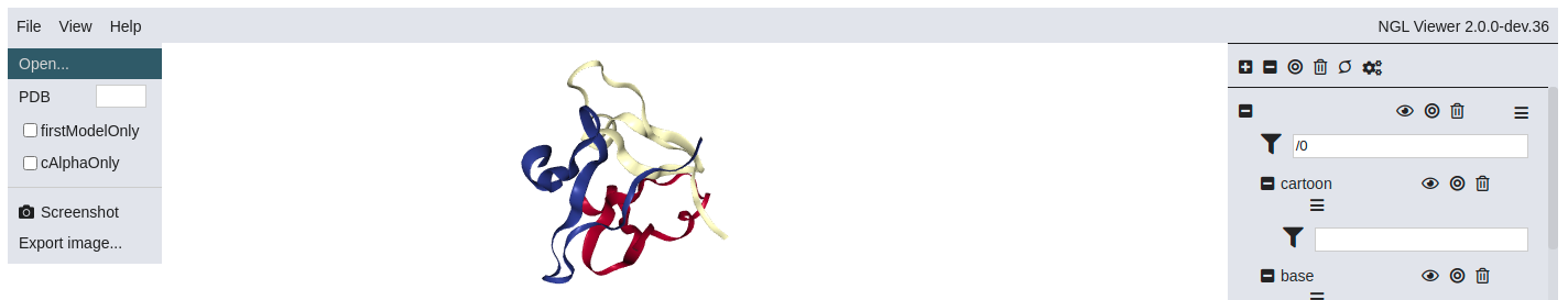
[52]:
view = get_pdb_nglviewer("1RFO", default_representation=False)
view.add_ribbon("protein")
view.center()
view
Sending GET request to https://files.rcsb.org/download/1RFO.pdb to fetch 1RFO's pdb file as a string.
This is what we need to display a single model:
clear all representations
and add the ribbon only on model N with the syntax
/N(atoms can have multiple possible positions based on the experimental data, which can be deposited in the PDB file as alternative models)
[53]:
view.clear()
view.add_ribbon("/0")
We can put this in a function.
[54]:
def show_one_model_only(view, model_id):
view.clear()
view.add_ribbon(f"/{model_id}")
Look how it reacts to your function calls.
[55]:
show_one_model_only(view, 1)
What if we let an IPyWidget do that for us? That’s how interact works! Read the documentation for more details, but the gist is:
interacttakes a function that accepts some parameters.Those parameters can be sent via changes in a widget (
model_id), or be manually defined as non-dynamic withfixed(parameter).interactdoes some magic to infer which kind of widget is best for each parameter. If you pass a tuple ofint(start, end), it will create a discrete slider, for example.Changing the state of the widget will result in calling that function with the new parameters. Since we are reacting on
view, you will see the changes in real time!
[56]:
from ipywidgets import interact, fixed
interact(show_one_model_only, view=fixed(view), model_id=(0, 9))
view
Change the value of the slider by dragging the widget!
Other interesting exercise is to change the type of representation with a widget. The full list is here.
[57]:
representations = ["backbone", "ball+stick", "line", "point", "ribbon"]
def change_representation(view, representation):
view.clear()
view.add_representation(representation)
view = view = get_pdb_nglviewer("1LEG")
interact(change_representation, view=fixed(view), representation=representations)
view
Sending GET request to https://files.rcsb.org/download/1LEG.pdb to fetch 1LEG's pdb file as a string.
What about color schemes? Same principle! Note that in this case these are arguments to a representation style. We are going to play with coloring schemes on ribbon.
[58]:
def change_coloring(view, coloring):
view.clear()
view.add_representation("ribbon", color_scheme=coloring)
view = get_pdb_nglviewer("1HND")
interact(change_coloring, view=fixed(view), coloring=nv.color.COLOR_SCHEMES[1:])
view
Sending GET request to https://files.rcsb.org/download/1HND.pdb to fetch 1HND's pdb file as a string.
Access the JavaScript layer
NGL is an incredibly powerful JavaScript library. NGLView exports the most commonly used bits to Python, which allows us to control certain things in a very convenient way. However, sometimes we need to leverage both layers (JS and Python) to achieve some advanced representations. To do so, we can use some private methods in nglview.NGLWidget. Namely:
nglview.NGLWidget._remote_call: Run a method on a NGL JS object, with positional argumentsargsand keyword argumentskwargs. You have to choose the target object first:target="Widget": The IPyWidget wrapper for the NGL Stage. Check public methods.target="Stage": Run any method onStage. List of methods.target="Viewer": Run any method onViewer. Check public methods.target="compList": Run any method oncompList, the list of loaded components in the stage. Maybe useful to query the JS list for a specific component.target="StructureComponent": Run any method onStructureComponent; each individual component. List of methods.
nglview.NGLWidget._execute_js_code: This will allow you to execute arbitrary JavaScript code. In that code, the JS counterpart of the IPyWidget can be referred bythis. The NGLStageinstance is available atthis.stage. It can be more powerful than_remote_callfor complex cases!
Let’s try some simple examples first.
[59]:
view = get_pdb_nglviewer("2G1T") # Human ABL1 kinase
view
Sending GET request to https://files.rcsb.org/download/2G1T.pdb to fetch 2G1T's pdb file as a string.
Let’s add some random text. This is possible via the addShape widget method. Some considerations:
Widget.addShaperequires arguments with a shape identifier or name (anystr) and a list of sublists, where each sublist contains the kind of “shape” and its arguments. See the function here.The arguments for each type shape can be checked on NGL documentation; e.g. for text. Use the search bar to find the corresponding
*Buffer.The arguments are passed without keywords, just the values, positionally.
Let’s add some red (encoded as RGB [1, 0, 0]) text (TeachOpenCADD) at the XYZ coordinates [60, 0, -20].
[60]:
view._remote_call(
"addShape",
target="Widget",
args=("redText", [["text", [60, 0, -20], [1, 0, 0], 10, "TeachOpenCADD"]]),
)
Note that this can be achieved in a similar way using _execute_js_code. The difference is how to pass arguments, which would need to be substituted in an f-string. Hopefully, for some simple cases, JS and Python share a similar syntax (e.g. lists and strings). Let’s add some more text, but now it will be blue and in a different position:
[61]:
view._execute_js_code("""
this.addShape("blueText", [["text", [60, 20, -20], [0, 0, 1], 10, "TeachOpenCADD"]])
""")
This might be cumbersome in some cases, but in others we don’t have a choice. For example, if we want to remove one of the shapes, we can only do it via _execute_js_code:
[62]:
view._execute_js_code("""
this.stage.removeComponent(this.stage.getComponentsByName("blueText").first)
""")
Debugging JavaScript code
You might be wondering how you can find the right JS command if autocomplete does not work and the documentation is tricky to follow. Your best chance is using the Developer Tools in your browser!
The trick is to export the NGL Widget, represented by this under the _execute_js_code context, to your browser tab context. To do so, execute this snippet:
[63]:
view._execute_js_code("document.nglview = this;")
If you open your Developer Tools console (Ctrl+Shift+J in Chrome, Ctrl+Shift+K in Firefox), you can type document.nglview there and inspect the object interactively:

For your convenience, you can also execute one more line in your JavaScript console to alias it to something quicker to type:
nv = document.nglview;
and inspect nv instead. Autocomplete with Tab should work as expected!
Tips and pitfalls:
Most of the interesting stuff will be under
nv.stage, likenv.stage.compList.The snippet you end up developing in the console will work as a
_execute_js_codesnippet as long as you replace backdocument.nglview(or your aliasnv) withthis.If you reload the NGL Widget from the notebook (e.g. by calling
nv.show_pdbid(...)again), you need to re-runview._execute_js_code("document.nglview = this;")The console allows for
non-;terminated lines, but make sure to end each line with;in the snippet.Javascript comments start with
//not#
Practical example: show residues around ligand
This is a popular operation we often perform while studying protein-ligand complexes, but NGLView does not expose that directly. NGL does offer that functionality, so we can still query JS for this!
Let’s open a kinase, e.g. EGFR, with an inhibitor bound. The PDB structure 2ITO seems to be bound by gefitinib with residue code IRE.
[64]:
view = get_pdb_nglviewer("2ITO")
view.center("IRE")
view
Sending GET request to https://files.rcsb.org/download/2ITO.pdb to fetch 2ITO's pdb file as a string.
[65]:
view._execute_js_code("""
// Get first (and only) loaded component: our protein-ligand system
var system = this.stage.compList[0];
// Store current selection, we will need it laer
var prevSele = system.selection.string;
// Set selection to our desired ligand
system.setSelection("IRE");
// Select all atoms within 5A from the ligand
var around = system.structure.getAtomSetWithinSelection(system.selection, 5.0);
// Extend selection so it includes full residues
var around_complete = system.structure.getAtomSetWithinGroup(around);
// Add representation for those atoms
system.addRepresentation("licorice", {sele: around_complete.toSeleString()});
// Restore selection to original one; otherwise changes won't be reflected
system.setSelection(prevSele)
""")
To parameterize this block of JS code you can use f-strings in a function! However, make sure to either:
Escape already present curly braces
{ }by doubling them:
- system.addRepresentation("licorice", {sele: around_complete.toSeleString()});
+ system.addRepresentation("licorice", {{sele: around_complete.toSeleString()}});
Split
{}-containing substrings from the f-string parts, thanks to implicit string concatenation:
js = (
f"""
// Get first (and only) loaded component: our protein-ligand system
var system = this.stage.compList[{index}];
// Store current selection, we will need it laer
var prevSele = system.selection.string;
// Set selection to our desired ligand
system.setSelection("{ligand}");
// Select all atoms within 5A from the ligand
var around = system.structure.getAtomSetWithinSelection(system.selection, {radius});
"""
# these extra quotes create two different strings: f-string above, regular string below
"""
// Extend selection so it includes full residues
var around_complete = system.structure.getAtomSetWithinGroup(around);
// Add representation for those atoms
system.addRepresentation("licorice", {sele: around_complete.toSeleString()});
// Restore selection to original one; otherwise changes won't be reflected
system.setSelection(prevSele)
"""
# In the end they are joined anyway, but _after_ the formatting has taken place :)
)
Knowing this, you can define show_residues_around like this:
[66]:
def show_residues_around(view, component_index=0, selection="ligand", radius=5.0):
js = (
f"""
// Get first (and only) loaded component: our protein-ligand system
var system = this.stage.compList[{component_index}];
// Store current selection, we will need it laer
var prevSele = system.selection.string;
// Set selection to our desired ligand
system.setSelection("{selection}");
// Select all atoms within 5A from the ligand
var around = system.structure.getAtomSetWithinSelection(system.selection, {radius});
"""
"""
// Extend selection so it includes full residues
var around_complete = system.structure.getAtomSetWithinGroup(around);
// Add representation for those atoms
system.addRepresentation("licorice", {sele: around_complete.toSeleString()});
// Restore selection to original one; otherwise changes won't be reflected
system.setSelection(prevSele)
"""
)
view._execute_js_code(js)
Let’s see if it works!
[67]:
view = get_pdb_nglviewer("1KSW")
show_residues_around(view)
view.center("ligand")
view
Sending GET request to https://files.rcsb.org/download/1KSW.pdb to fetch 1KSW's pdb file as a string.
This way of working with NGL opens a world of possibilities! The issues labeled as Q&A in the nglview repository often resort this technique, and now you will be able to know what’s going on!
Troubleshooting tips
The Jupyter ecosystem is vast and changes rapidly. Keeping up-to-date with the latest additions is tricky and resource consuming, so ending up with a broken NGLView installation is not uncommon. The following packages might affect the functionality of NGLView. If one of them had a recent version change (specially major versions, like Jupyter Lab 2 -> Jupyter Lab 3), that might be one of the possible explanations for the errors you are seeing:
jupyterjupyterlabnotebookipywidgetsnglviewitself
Tip: If
nglviewcan be imported but you don’t see the canvas fornv.demo(), check the Developer Tools console (Ctrl+Shift+J in Chrome, Ctrl+Shift+K in Firefox) for error messages! 404 errors trying to load the JS NGL libraries are one of the most common ones. Check the steps below to troubleshoot!
Check which Jupyter platform you are working from
While the community transitions from Jupyter Notebook to Jupyter Lab, these alternative frontends for our beloved notebooks will coexist for a while, making everything a bit more confusing. Which one are you using? Check the table below.
Application |
Package name |
Shell command |
URL style |
Features |
|---|---|---|---|---|
Jupyter Notebook |
|
|
|
One notebook per tab; Less resource intensive; Legacy project |
Jupyter Lab v2 |
|
|
|
Multiple notebooks per tab; You can compose complex interfaces; Consumes more resources; Extensions must be built on the machine before installation |
Jupyter Lab v3 |
|
|
|
No need to build extensions |
Jupyter Classic |
|
|
|
Same UI style as |
As a result, installing nglview on your machine involves different step depending on which Jupyter UI you are going to use.
How to install nglview, the right way
If you didn’t know about the subtle differences explained above, there’s a chance you have several instances of nglview installed in your computer. Having both conda and pip available makes it more difficult, specially if you mix system installations with environment ones. Our advice is that you create a fresh environment for each project you work on, and specify their dependencies explicitly.
To get to that clean slate you might need to delete some files that will interfere with the environment-specific setting.
Jupyter Notebook
conda install -c conda-forge nglview
nglview install
nglview enable
If this does not work, there’s a chance Jupyter Notebook is finding other installations of nglview that interfere with the expected JavaScript libraries. The paths that Jupyter will check are listed with jupyter --paths.
To make sure the right ones are loaded (the ones in the active environment), you might need to delete some directories:
For Linux and Mac OS:
# User-level widgets
rm -rf ~/.local/share/jupyter/nbextensions/nglview-js-widgets/
# Global conda widgets
rm -rf $(conda info --base)/share/jupyter/nbextensions/nglview-js-widgets/
For Windows:
del %APPDATA%\jupyter\nbextensions\nglview-js-widgets
del %_CONDA_ROOT%\share\jupyter\nbextensions\nglview-js-widgets
Then, close Jupyter Notebook tabs and the command-line process, and relaunch. If this didn’t work:
Make sure the locations shown by
jupyter --pathsdo not contain NGL files under<prefix>/share/jupyter/nbextensions/nglview-js-widgets/.Run
conda remove nglviewand / orpip uninstall nglviewand start again.Hard-reload the browser tab with Ctrl+Shift+R.
Check this excellent FAQ for more ideas.
Jupyter Lab (v2 style)
Since Jupyter Lab uses a different extension system, it doesn’t suffer from the path precedence issues shown above. However, you need to make sure the extension was installed and built:
conda install -c conda-forge nglview
jupyter labextension install @jupyter-widgets/jupyterlab-manager nglview-js-widgets
Jupyter Lab (v3+ style)
Jupyter Lab v3 and above use a nice trick to precompile the JavaScript libraries, so you will only need to install nglview with your favourite package manager.
conda install -c conda-forge nglview
Discussion
NGLView is an incredibly powerful widget with a lot of features already accessible from the Python interface. But it’s easy to miss the potential of the underlying JavaScript library! We hope you could see some of the possibilities available and that you’ve learned the tools you need to use to get there and beyond. If you are interested in some more examples of advanced uses, check the links below.
Quiz
NGLView is now part of your CADD toolbox. Here you have some interesting exercises:
Load one of the structures for ABL1 (available at KLIFS.net), without downloading anything manually. Check talktorial
T013for more details about KLIFS!Color the pocket residues in a different tone for easy visual identification.
Show the side chains of those residues that are potentially interacting with the ligand, if present.
Create a small interface that lists all ABL1 structures available at KLIFS. Clicking on their PDB ID should load the structure and the visualizations discussed above.