T016 · Protein-ligand interactions
Note: This talktorial is a part of TeachOpenCADD, a platform that aims to teach domain-specific skills and to provide pipeline templates as starting points for research projects.
Authors:
Jaime Rodríguez-Guerra 2019-2020, Volkamer lab
Michele Wichmann, 2019-2020, Charité/FU Berlin
Yonghui Chen, 2020, Volkamer lab
Talia B. Kimber, 2020, Volkamer lab
Andrea Volkamer, 2020, Volkamer lab
Aim of this talktorial
In this talktorial, we focus on protein-ligand interactions. Understanding such interactions, which are driving molecular recognition, are fundamental in drug design.
To this end, we use two Python tools: the first one, called the Protein–Ligand Interaction Profiler, or PLIP, to get insight into protein-ligand interactions for any sample complex and the second, NGLView, to visualize the interactions in 3D.
Contents in Theory
Protein-ligand interactions
PLIP: Protein–Ligand Interaction Profiler
Web service
Algorithm
Visualization: complex and interactions
Contents in Practical
PDB complex: example with EGFR
Profiling protein-ligand interactions using PLIP
Table of interaction types
Visualization with NGLView
Analysis of interactions
References
Review on protein-ligand interactions (Int. J. Mol. Sci. (2016), 17, 144)
A systematic analysis of non-covalent interactions in the PDB database (M. Med. Chem. Commun. (2017), 8, 1970-1981)
A chapter about how protein–ligand interactions are key for drug action (in Klebe G. (eds) Drug Design. Springer, Berlin, Heidelberg.)
Tools
NGLView, the interactive molecule visualizer for Jupyter notebooks (Bioinformatics (2018), 34, 1241–124)
PLIP, the Protein–Ligand Interaction Profiler (Nucl. Acids Res. (2015), 43, W1, W443-W447)
[1]:
import sys

if "google.colab" in sys.modules:
    %pip install teachopencadd --no-deps -q
    !teachopencadd -d 16
    %pip uninstall teachopencadd -y -q
    %pip install -qr requirements.txt
    %conda install openbabel plip -c conda-forge -y
Theory
Protein-ligand interactions
Ligand binding is mainly governed by non-covalent interactions between the ligand and the surface of the protein pocket or the protein-protein interface. This process is a function of electrostatic and shape complementarities, induced fitting, desolvation processes and more.
Some quotes from the literature:
Adapted from José L. Medina-Franco, Oscar Méndez-Lucio, Karina Martinez-Mayorga:
Understanding protein–ligand interactions (PLIs) and protein–protein interactions (PPIs) is at the core of molecular recognition and has a fundamental role in many scientific areas. PLIs and PPIs have a broad area of practical applications in drug discovery including but not limited to molecular docking, structure-based design, virtual screening of molecular fragments, small molecules, and other types of compounds, clustering of complexes, and structural interpretation of activity cliffs, to name a few.
These interactions can be rationalized in several ways, which for example opens the door to systematic analysis of the docking solutions.
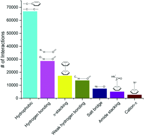
Figure 1 : Frequency of non-colavent interactions. Out of 750,873 ligand–protein atom pairs extracted from complexes from the PDB data base, the 100 most frequent pairs can be grouped into seven interaction types, as shown in the figure (taken from the paper by de Freitas and Schapira, A systematic analysis of atomic protein–ligand interactions in the PDB, 2017).
There are several programs to assess protein-ligand interactions in an automated way.
For example, the Kinase-Ligand Interaction Fingerprints and Structures database (KLIFS) is a kinase centric tool with a freely available web service. More details can be found in Talktorial T012: “Data acquisition from KLIFS”.
PLIP: Protein–Ligand Interaction Profiler
For a more general set of proteins, PLIP is also popular thanks to its publicly available webserver and free-to-use Python library.
PLIP: web service
The PLIP web service is a freely available tool which allows to exhibit protein-ligand interactions from any PDB structure as shown in Figure 2 below.
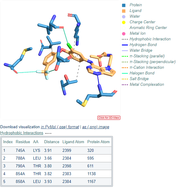
Figure 2 : Visualization of protein-ligand interactions generated by the PLIP web service. The example displays an EGFR kinase complex, associated PDB ID 3POZ. The figure, a snapshot from the web service result, shows
the 3D plot of the protein and the ligand and the different interactions types detected (see legend on the right).
an example table describing the hydrophobic interactions between atoms from the protein and the ligand.
PLIP: algorithm
For each binding site, the PLIP algorithm considers the atoms from the protein and the ligand only if they lie within a certain distance cutoff. Once the protein and ligand atoms that potentially interact are identified, non-covalent interactions can be detected, such as:
hydrophobic interactions
hydrogen bonds
aromatic stacking
pi-cation interactions
salt bridges
water-bridged hydrogen bonds
halogen bonds
They are defined using geometry rules, such as distance and angle thresholds.
The supporting information accompanying the manuscript (Nucl. Acids Res. (2015), 43, W1, W443-W447) describes the binding site detection and protein-ligand interactions in detail, please see the PDF document below.
[4]:
from IPython.display import display, HTML

pdf_url = "https://www.ncbi.nlm.nih.gov/pmc/articles/PMC4489249/bin/supp_gkv315_nar-00254-web-b-2015-File003.pdf"

# Construct the URL for the Google Docs Viewer service
viewer_url = f"https://docs.google.com/viewer?url={pdf_url}&embedded=true"

# Display the PDF using the HTML <iframe> tag
display(
    HTML(
        f'<iframe src="{viewer_url}" width="900" height="600" frameborder="0" allowfullscreen></iframe>'
    )
)
/opt/miniconda3/envs/T016_3100/lib/python3.10/site-packages/IPython/core/display.py:475: UserWarning: Consider using IPython.display.IFrame instead
  warnings.warn("Consider using IPython.display.IFrame instead")
Visualization: complex and interactions
We will use nglview for visualization. It’s a web-based molecular viewer that can be run on Jupyter notebooks. We will first use it in a basic way to visualize a complex of interest. Then, we will make use of ipywidgets layouts to visualize protein-ligand interactions.
More details can be found in Talktorial T017 on advanced NGLview & widget usage.
Practical
[5]:
# Import libraries
from pathlib import Path
import time
import warnings

warnings.filterwarnings("ignore")

import pandas as pd
import nglview as nv
from pypdb.clients.pdb.pdb_client import get_pdb_file

# import openbabel
import numpy as np
import matplotlib.pyplot as plt
from matplotlib import colors
from plip.structure.preparation import PDBComplex
from plip.exchange.report import BindingSiteReport

from opencadd.structure.core import Structure
2025-12-22 13:54:22,369 [WARNING] [TRJ.py:151] MDAnalysis.coordinates.AMBER: netCDF4 is not available. Writing AMBER ncdf files will be slow.
[6]:
def get_structure(pdb_id):
    # download the PDB file content.
    pdb_file_content = get_pdb_file(pdb_id)
    # create an nglview structure object from the content
    structure = nv.TextStructure(pdb_file_content, ext="pdb")
    return structure


def get_pdb_nglviewer(pdb_id, default_representation=True, gui=False):
    structure = get_structure(pdb_id)
    # set structure viewer
    nglviewer = nv.show_file(structure, default_representation=default_representation, gui=gui)
    return nglviewer
[7]:
# Absolute path
HERE = Path(_dh[-1])
DATA = HERE / "data"
PDB complex: example with EGFR
As a test case for this notebook, we choose the EGFR kinase. The considered PDB structure is given by the ID 3POZ. Let’s use nglview to visualize the structure in a notebook cell.
Note: the complex can easily be changed by adapting the PDB ID in the cell below.
[8]:
pdb_id = "3poz"
We now fetch the PDB structure file from the PDB using opencadd.structure.superposition. More details can be found in Talktorial T008 for protein data acquisition.
[9]:
pdb_file = Structure.from_pdbid(pdb_id)
# Download it to file for later use
pdb_file.write(DATA / f"{pdb_id}.pdb")
Show the complex based on PDB ID
[10]:
ngl_viewer = get_pdb_nglviewer(pdb_id)
# add the ligands
ngl_viewer.add_representation(repr_type="ball+stick", selection="hetero and not water")
# center view on binding site
ngl_viewer.center("ligand")
ngl_viewer
Sending GET request to https://files.rcsb.org/download/3poz.pdb to fetch 3poz's pdb file as a string.
[11]:
# render a static image
ngl_viewer.render_image(trim=True, factor=2);
[29]:
ngl_viewer._display_image()
[29]:
Profiling protein-ligand interactions using PLIP
PLIP offers a webserver for automated analysis, but unfortunately there is no API. We could try to use the HTML forms as if we were using the standard web UI, but since the library itself is Python-3 ready and very easy to install with pip, we can just use it locally for simplicity.
PLIP takes PDB files as input, so we can pass the PDB file to PLIP and let it do its magic. The BindingSiteReport class processes each detected binding site in PDBComplex and creates an object with the (eight) fields we are interested in, namely
hydrophobic interaction :
hydrophobichydrogen bond :
hbondwater bridge :
waterbridgesalt bridge :
saltbridge\(\pi\)-stacking (parallel and perpendicular) :
pistacking\(\pi\)- cation :
picationhalogen bond :
halogenmetal complexation :
metal
These fields are divided in <field>_features (containing column names) and <field>_info (containing the actual records). If we iterate over the object retrieving the correct attribute name with getattr(), we can compose a dictionary that can be passed to a pandas.DataFrame for nice overviews.
This dictionary is composed of two levels:
First level is the detected binding sites.
For each binding site, we have one more sub-dictionary containing eight lists, one for each specific interaction.
Each list will contain the column names in the first row, and the data (if available) in the following.
[13]:
def retrieve_plip_interactions(pdb_file):
    """
    Retrieves the interactions from PLIP.

    Parameters
    ----------
    pdb_file :
        The PDB file of the complex.

    Returns
    -------
    dict :
        A dictionary of the binding sites and the interactions.
    """
    protlig = PDBComplex()
    protlig.load_pdb(pdb_file)  # load the pdb file
    for ligand in protlig.ligands:
        protlig.characterize_complex(ligand)  # find ligands and analyze interactions
    sites = {}
    # loop over binding sites
    for key, site in sorted(protlig.interaction_sets.items()):
        binding_site = BindingSiteReport(site)  # collect data about interactions
        # tuples of *_features and *_info will be converted to pandas DataFrame
        keys = (
            "hydrophobic",
            "hbond",
            "waterbridge",
            "saltbridge",
            "pistacking",
            "pication",
            "halogen",
            "metal",
        )
        # interactions is a dictionary which contains relevant information for each
        # of the possible interactions: hydrophobic, hbond, etc. in the considered
        # binding site. Each interaction contains a list with
        # 1. the features of that interaction, e.g. for hydrophobic:
        # ('RESNR', 'RESTYPE', ..., 'LIGCOO', 'PROTCOO')
        # 2. information for each of these features, e.g. for hydrophobic
        # (residue nb, residue type,..., ligand atom 3D coord., protein atom 3D coord.)
        interactions = {
            k: [getattr(binding_site, k + "_features")] + getattr(binding_site, k + "_info")
            for k in keys
        }
        sites[key] = interactions
    return sites
We create the dictionary for the complex of interest:
[14]:
interactions_by_site = retrieve_plip_interactions(f"{DATA}/{pdb_id}.pdb")
Let’s see how many binding sites are detected:
[15]:
print(
    f"Number of binding sites detected in {pdb_id} : "
    f"{len(interactions_by_site)}\n"
    f"with {interactions_by_site.keys()}"
)
# NBVAL_CHECK_OUTPUT
Number of binding sites detected in 3poz : 4
with dict_keys(['03P:A:1023', 'SO4:A:1', 'SO4:A:2', 'SO4:A:3'])
In this case, the first binding site containing ligand 03P will be further investigated.
[16]:
index_of_selected_site = 0
selected_site = list(interactions_by_site.keys())[index_of_selected_site]
print(selected_site)
03P:A:1023
Table of interaction types
We can construct a pandas.DataFrame for a binding site and particular interaction type.
[17]:
def create_df_from_binding_site(selected_site_interactions, interaction_type="hbond"):
    """
    Creates a data frame from a binding site and interaction type.

    Parameters
    ----------
    selected_site_interactions : dict
        Precaluclated interactions from PLIP for the selected site
    interaction_type : str
        The interaction type of interest (default set to hydrogen bond).

    Returns
    -------
    pd.DataFrame :
        DataFrame with information retrieved from PLIP.
    """

    # check if interaction type is valid:
    valid_types = [
        "hydrophobic",
        "hbond",
        "waterbridge",
        "saltbridge",
        "pistacking",
        "pication",
        "halogen",
        "metal",
    ]

    if interaction_type not in valid_types:
        print("!!! Wrong interaction type specified. Hbond is chosen by default!!!\n")
        interaction_type = "hbond"

    df = pd.DataFrame.from_records(
        # data is stored AFTER the column names
        selected_site_interactions[interaction_type][1:],
        # column names are always the first element
        columns=selected_site_interactions[interaction_type][0],
    )
    return df
Hydrophobic interactions
In the next cell, we show the hydrophobic interactions from the selected binding site.
[18]:
create_df_from_binding_site(interactions_by_site[selected_site], interaction_type="hydrophobic")
[18]:
| RESNR | RESTYPE | RESCHAIN | RESNR_LIG | RESTYPE_LIG | RESCHAIN_LIG | DIST | LIGCARBONIDX | PROTCARBONIDX | LIGCOO | PROTCOO | |
|---|---|---|---|---|---|---|---|---|---|---|---|
| 0 | 745 | LYS | A | 1023 | 03P | A | 3.91 | 2398 | 320 | (18.317, 32.25, 10.052) | (20.469, 34.989, 8.267) |
| 1 | 788 | LEU | A | 1023 | 03P | A | 3.66 | 2383 | 595 | (18.404, 30.743, 6.486) | (18.317, 33.573, 4.169) |
| 2 | 790 | THR | A | 1023 | 03P | A | 3.80 | 2397 | 611 | (16.476, 34.203, 10.862) | (12.875, 33.449, 9.914) |
| 3 | 854 | THR | A | 1023 | 03P | A | 3.82 | 2382 | 1138 | (18.135, 32.543, 11.422) | (17.798, 28.992, 12.797) |
| 4 | 858 | LEU | A | 1023 | 03P | A | 3.93 | 2383 | 1167 | (18.404, 30.743, 6.486) | (22.084, 30.736, 5.093) |
As you can notice, this table matches the figure in the Theory part of the notebook.
Hydrogen interactions
If hydrogen interactions are of interest, the table can be generated as follow:
[19]:
create_df_from_binding_site(interactions_by_site[selected_site], interaction_type="hbond")
[19]:
| RESNR | RESTYPE | RESCHAIN | RESNR_LIG | RESTYPE_LIG | RESCHAIN_LIG | SIDECHAIN | DIST_H-A | DIST_D-A | DON_ANGLE | PROTISDON | DONORIDX | DONORTYPE | ACCEPTORIDX | ACCEPTORTYPE | LIGCOO | PROTCOO | |
|---|---|---|---|---|---|---|---|---|---|---|---|---|---|---|---|---|---|
| 0 | 793 | MET | A | 1023 | 03P | A | False | 2.01 | 2.96 | 163.57 | True | 629 | Nam | 2404 | Nar | (13.371, 34.064, 15.005) | (10.667, 33.654, 16.145) |
Halogen interactions
Let’s also have a look at halogen interactions:
[20]:
create_df_from_binding_site(interactions_by_site[selected_site], interaction_type="halogen")
[20]:
| RESNR | RESTYPE | RESCHAIN | RESNR_LIG | RESTYPE_LIG | RESCHAIN_LIG | SIDECHAIN | DIST | DON_ANGLE | ACC_ANGLE | DON_IDX | DONORTYPE | ACC_IDX | ACCEPTORTYPE | LIGCOO | PROTCOO | |
|---|---|---|---|---|---|---|---|---|---|---|---|---|---|---|---|---|
| 0 | 766 | MET | A | 1023 | 03P | A | False | 3.60 | 167.05 | 118.86 | 2389 | F | 431 | O2 | (14.283, 28.118, 6.395) | (12.164, 26.835, 3.777) |
| 1 | 788 | LEU | A | 1023 | 03P | A | False | 3.23 | 159.67 | 108.02 | 2396 | Cl | 592 | O2 | (15.676, 34.766, 8.319) | (14.792, 37.053, 6.216) |
| 2 | 790 | THR | A | 1023 | 03P | A | True | 3.47 | 171.27 | 103.84 | 2388 | F | 610 | O3 | (13.867, 29.356, 8.056) | (11.467, 31.629, 9.124) |
Visualization with NGLView
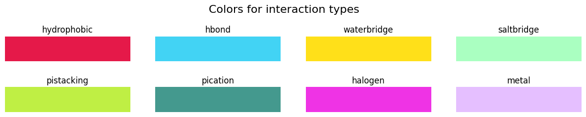
Now, let’s try to represent those interactions in the NGL viewer. We can draw cylinders between the interaction points (LIGCOO and PROTCOO in the pandas.DataFrame) and color-code them as shown in color_map, which uses RGB tuples.
[21]:
color_map = {
    "hydrophobic": [0.90, 0.10, 0.29],
    "hbond": [0.26, 0.83, 0.96],
    "waterbridge": [1.00, 0.88, 0.10],
    "saltbridge": [0.67, 1.00, 0.76],
    "pistacking": [0.75, 0.94, 0.27],
    "pication": [0.27, 0.60, 0.56],
    "halogen": [0.94, 0.20, 0.90],
    "metal": [0.90, 0.75, 1.00],
}
Let’s see what these RGB colors correspond to:
[27]:
fig, axs = plt.subplots(nrows=2, ncols=4, figsize=(15, 2))
plt.subplots_adjust(hspace=1)
fig.suptitle("Colors for interaction types", size=16, y=1.2)

for ax, (interaction, color) in zip(fig.axes, color_map.items()):
    ax.imshow(np.zeros((1, 5)), cmap=colors.ListedColormap(color_map[interaction]))
    ax.set_title(interaction, loc="center")
    ax.set_axis_off()
plt.show()
Define a helper function to show the interactions.
[23]:
def show_interactions_3d(
    pdb_id, selected_site_interactions, highlight_interaction_colors=color_map
):
    """
    3D visualization of protein-ligand interactions.

    Parameters
    ----------
    pdb_id : str
        The pdb ID of interest.
    selected_site_interactions : dict
        Precaluclated interactions from PLIP for the selected site
    highlight_interaction_colors : dict
        The colors used to highlight the different interaction types.

    Returns
    -------
    NGL viewer with explicit interactions given by PLIP.
    """

    # Create NGLviewer
    viewer = nv.NGLWidget(height="600px", default=True, gui=True)
    # Add protein
    prot_component = viewer.add_pdbid(pdb_id)
    # Add the ligands
    viewer.add_representation(repr_type="ball+stick", selection="hetero and not water")

    interacting_residues = []
    for interaction_type, interaction_list in selected_site_interactions.items():
        color = highlight_interaction_colors[interaction_type]
        if len(interaction_list) == 1:
            continue
        df_interactions = pd.DataFrame.from_records(
            interaction_list[1:], columns=interaction_list[0]
        )
        for _, interaction in df_interactions.iterrows():
            name = interaction_type
            # add cylinder between ligand and protein coordinate
            viewer.shape.add_cylinder(
                interaction["LIGCOO"],
                interaction["PROTCOO"],
                color,
                [0.1],
                name,
            )
            interacting_residues.append(interaction["RESNR"])
    # Display interacting residues
    res_sele = " or ".join([f"({r} and not _H)" for r in interacting_residues])
    res_sele_nc = " or ".join([f"({r} and ((_O) or (_N) or (_S)))" for r in interacting_residues])
    prot_component.add_ball_and_stick(sele=res_sele, colorScheme="chainindex", aspectRatio=1.5)
    prot_component.add_ball_and_stick(sele=res_sele_nc, colorScheme="element", aspectRatio=1.5)
    # Center on ligand
    viewer.center("ligand")
    return viewer
[24]:
viewer_3d = show_interactions_3d(pdb_id, interactions_by_site[selected_site])
viewer_3d
[25]:
viewer_3d.render_image(trim=True, factor=2, transparent=True);
[28]:
viewer_3d._display_image()
[28]:
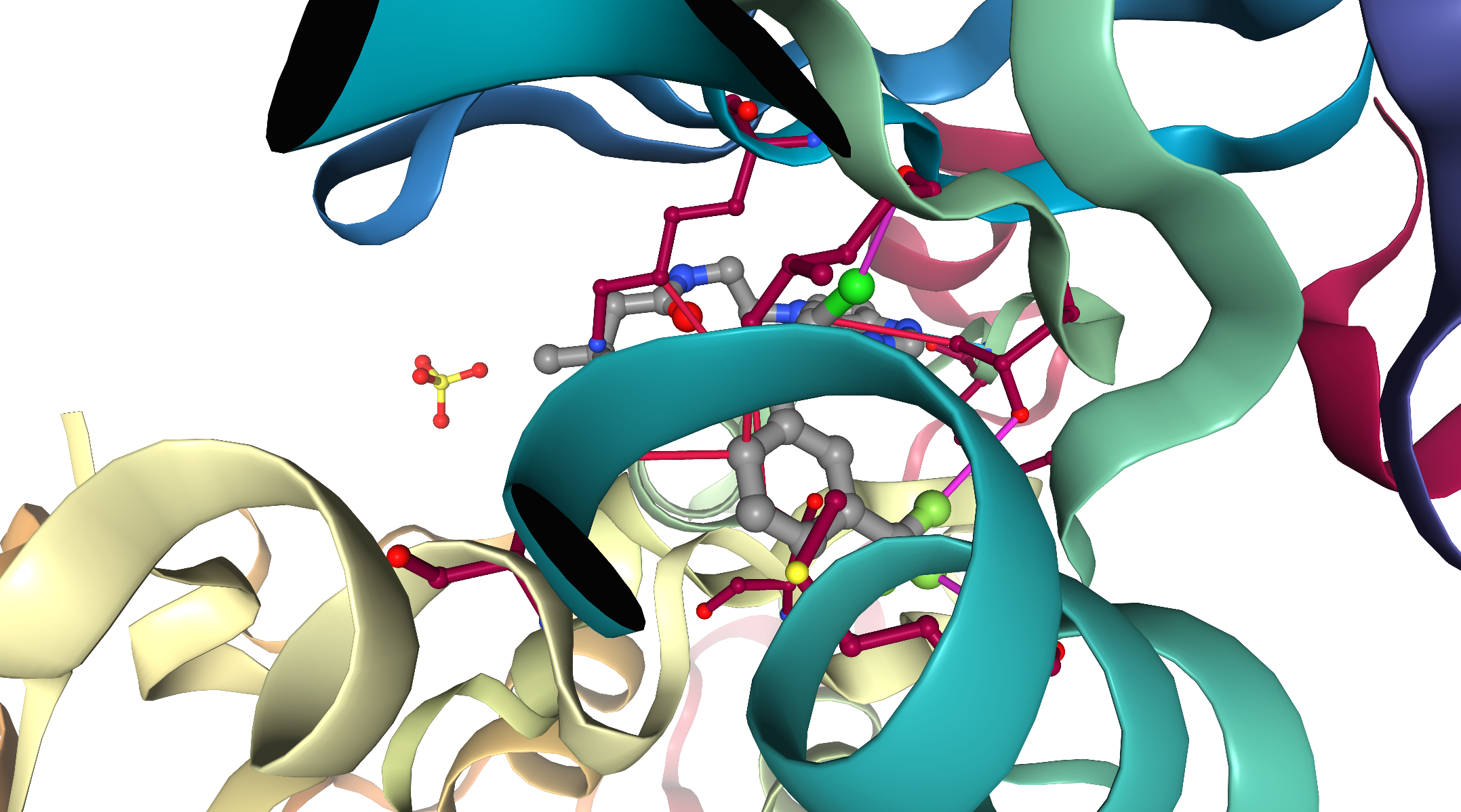
Analysis of interactions
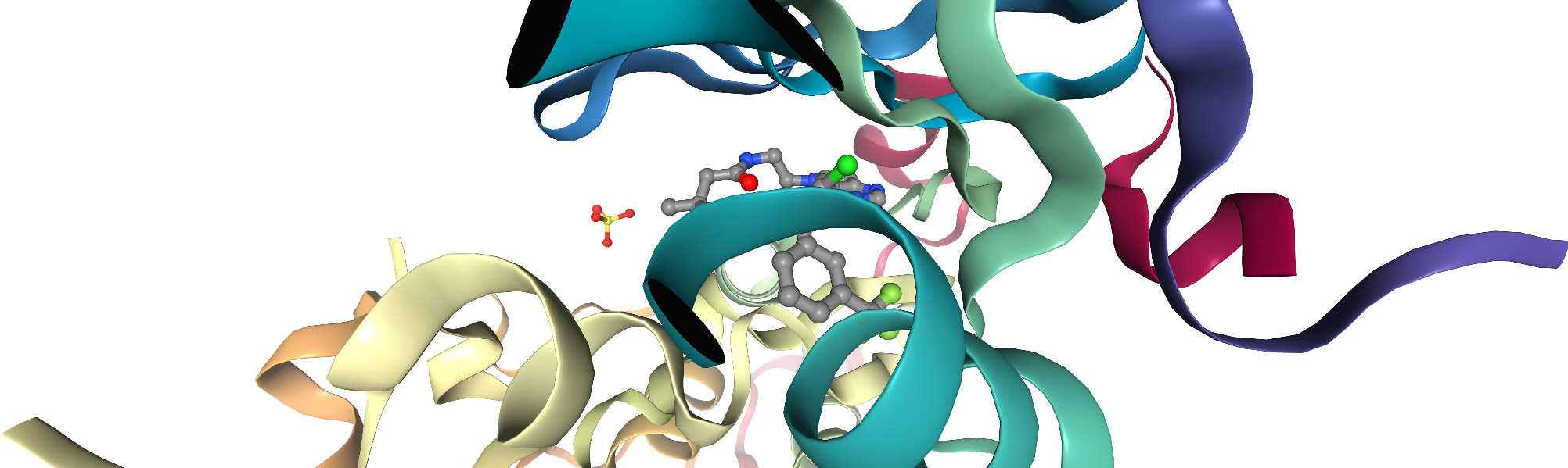
As we can see in the NGL viewer, PLIP manages to identify different interactions between the protein and the ligand in the binding site, for our kinase example (3poz):
The typical hinge hydrogen binding with methionine residue MET793.
Hydrophobic interactions with the following residues:
LYS745
LEU788
THR790
THR854
LEU858
Halogen interactions with residues:
MET766
LEU788
THR790
Note that for example the hinge interaction is equally identified in KLIFS, see 3poz KLIFS fingerprint, while the hydrophobic interactions identified with PLIP are only a subset of those in KLIFS. Halogen interactions are not explicitly annotated in KLIFS.
All the identified interactions in NGLview do indeed correspond to the table of interactions generated above.
Discussion
In this talktorial we have learned about protein-ligand interactions, more specifically in the context of the Protein–Ligand Interaction Profiler, or PLIP for short. We created a DataFrame to depict the interactions in a table. Furthermore, we made use of the NGL viewer to visualize these interactions in 3D, which require a good amount of web technologies, mainly based around the NGL viewer itself and ipywidgets layouts.
Quiz
Do some interactions seem more important than others?
What’s the main difference between hydrophobic interactions and hydrogen bonds? How are they similar?
What can be a considerable advantage of using PLIP over KLIFS?